Graph

Author

Marc Garel & Fabrice Armougom

I-Use of ggplot packages to perform smart plot

ggplot2 is a powerfull packages to make a very smart graph “ready to use” for publication. gg means grammar and graph, a concept which describe a graph using grammar. This package belong to tidyverse according to “dplyr”. According to the ggplot2 concept, a graph can be divided into different basic parts:Plot = data + Aesthetics + Geometry

data : data frame
aesthetics : allows to indicate the x and y variables. It can also be used to control the color, size and shape of the points, etc…
geometry : corresponds to the type of graph (histogram, box plot, line plot, …..)

How to build a graph

Scatter plot

# if not alraedy done load library ggplot2
library(ggplot2)
library(dplyr)


Attaching package: 'dplyr'

The following objects are masked from 'package:stats':

    filter, lag

The following objects are masked from 'package:base':

    intersect, setdiff, setequal, union

data(iris)
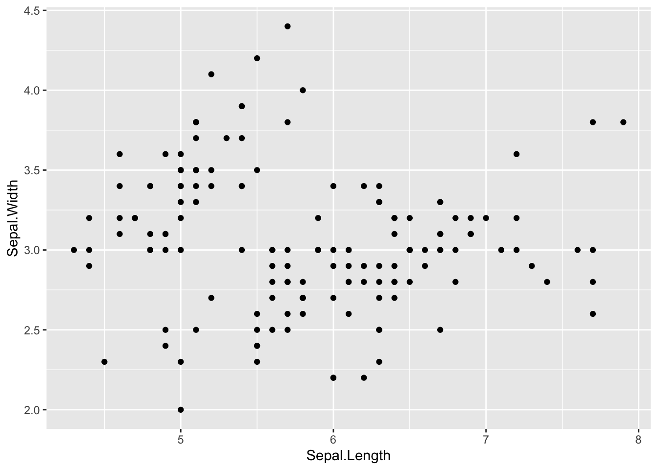
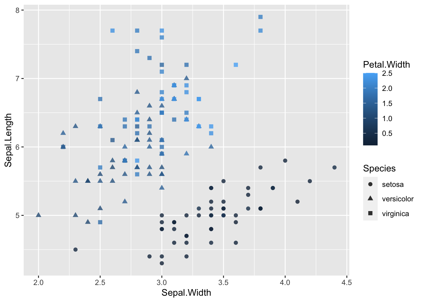
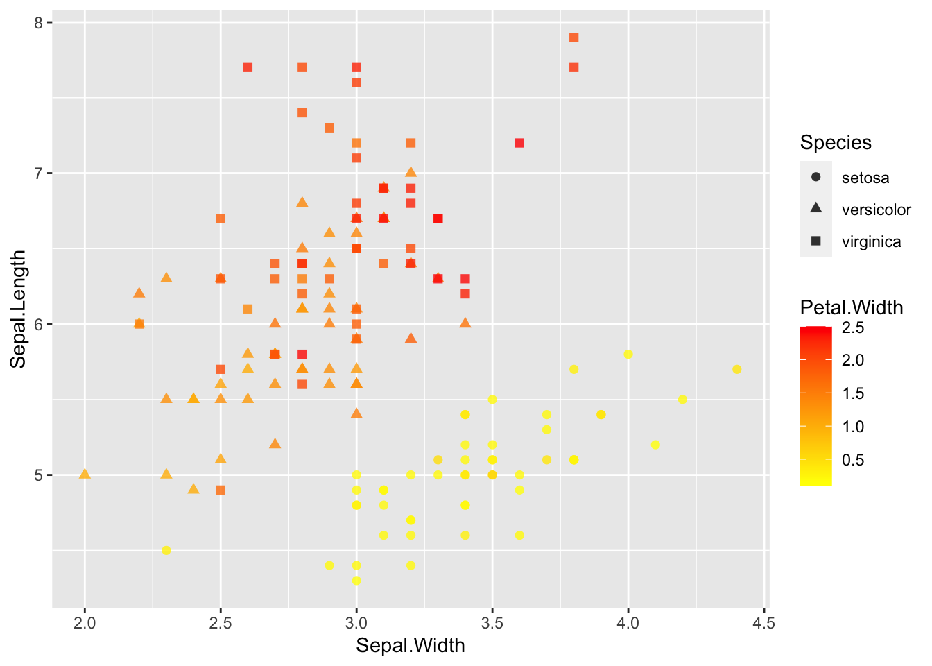
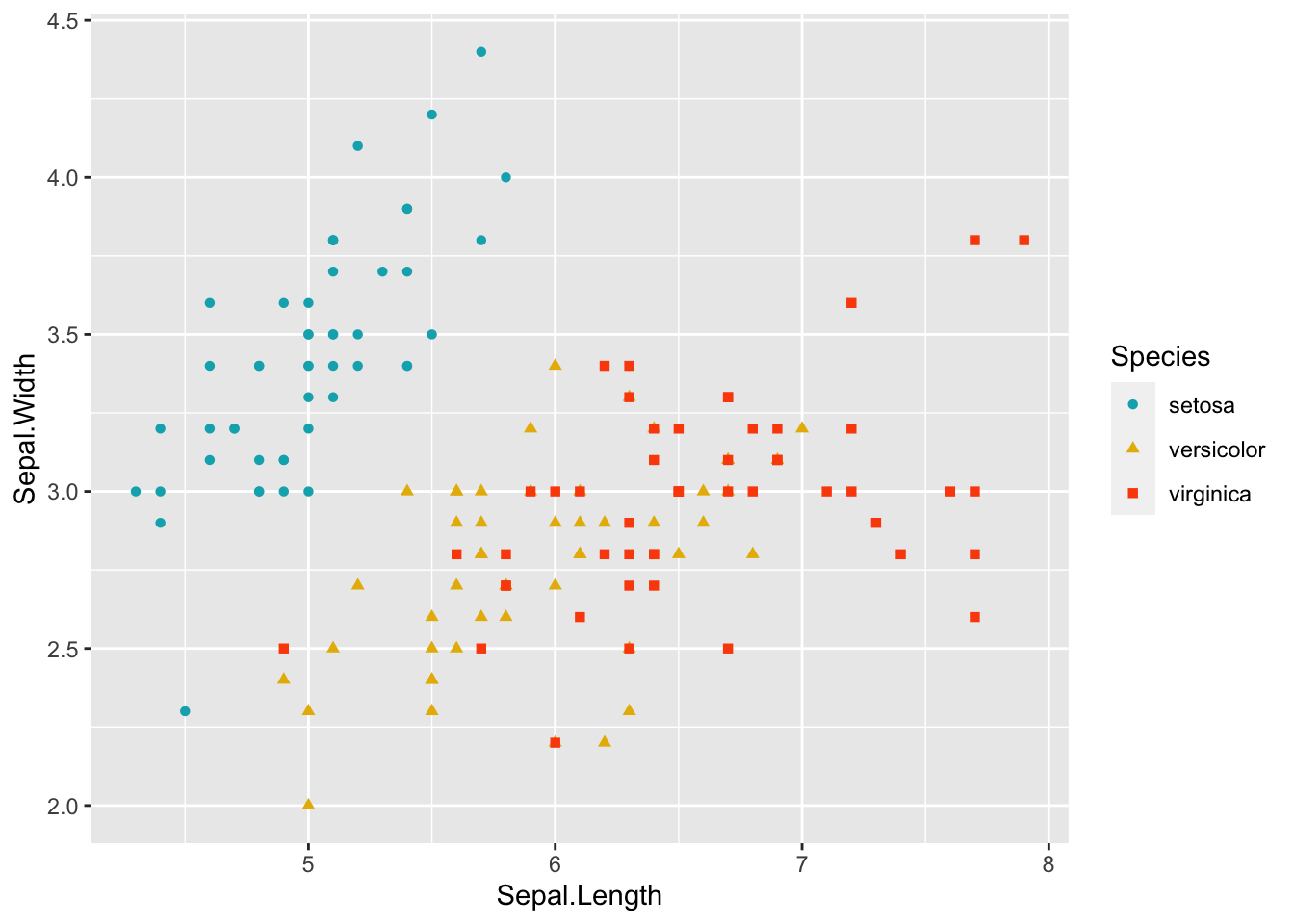
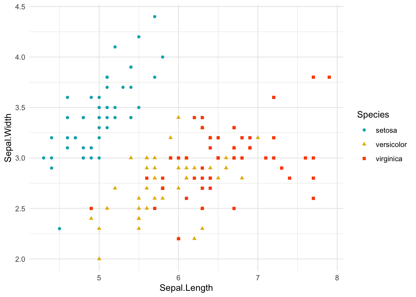
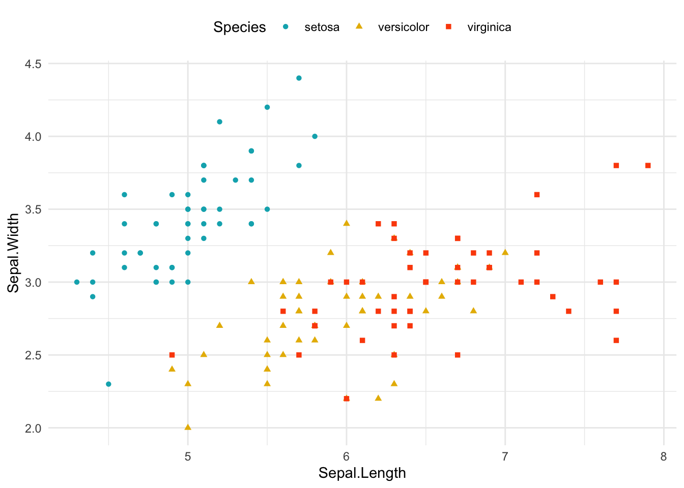
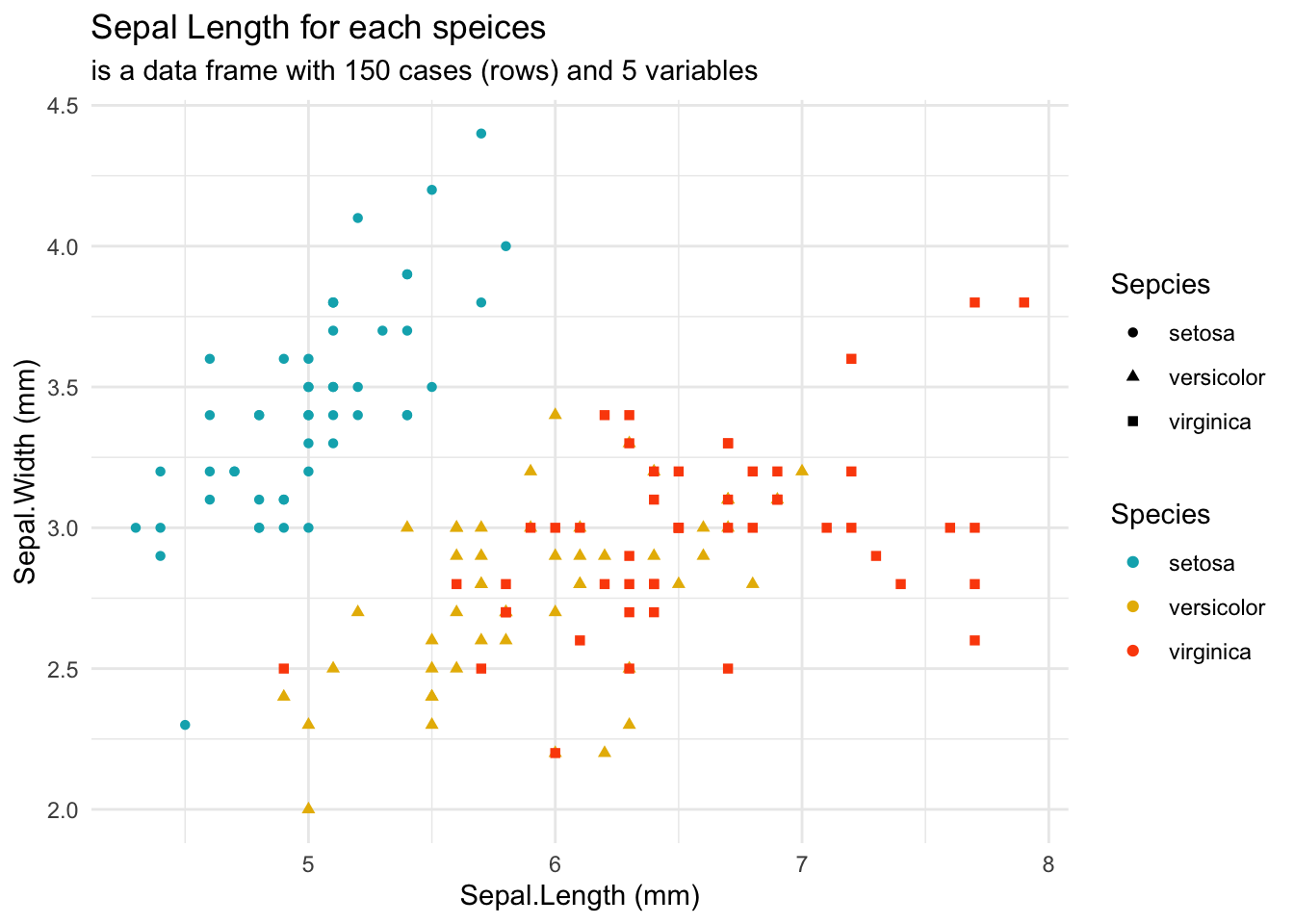
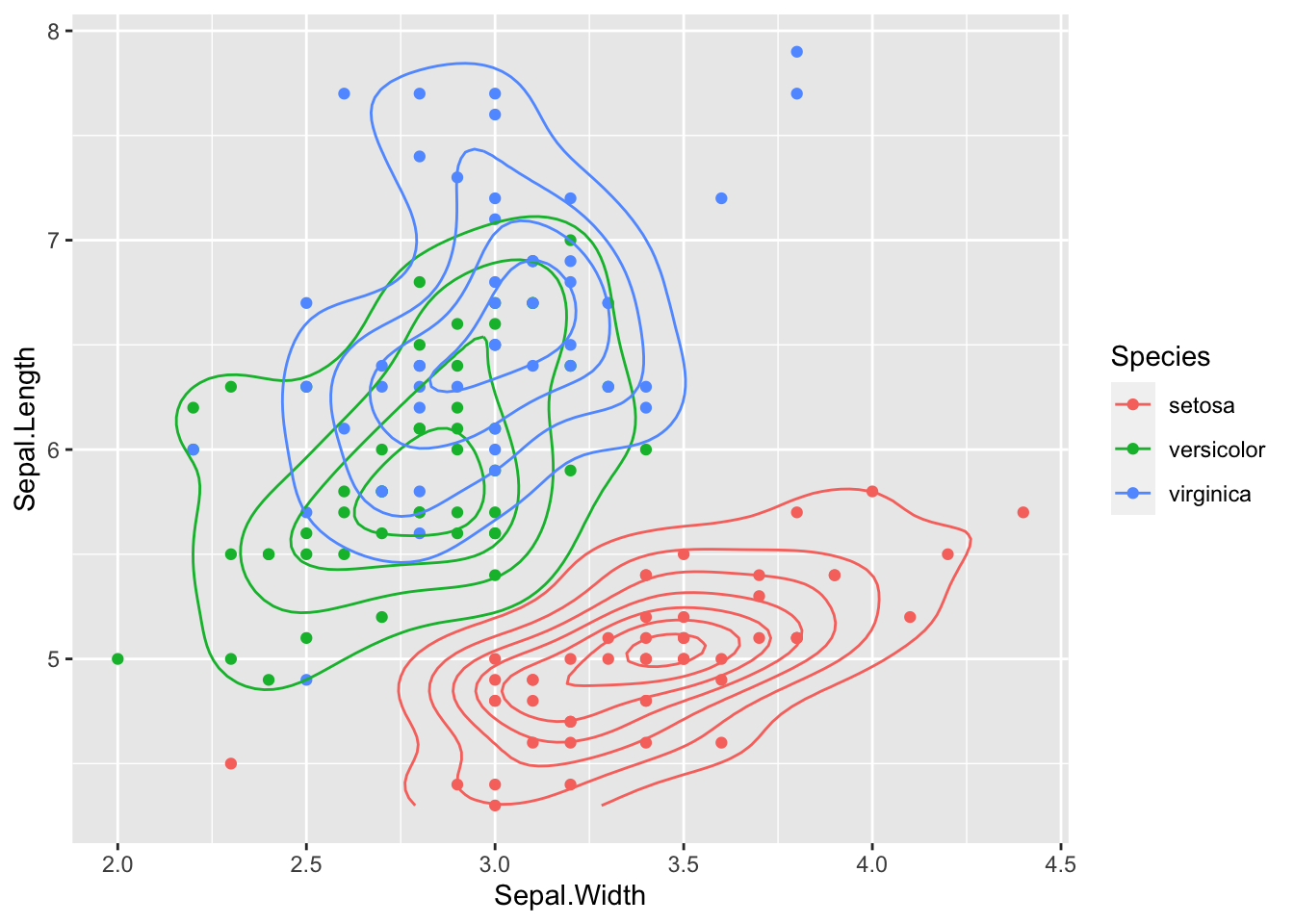
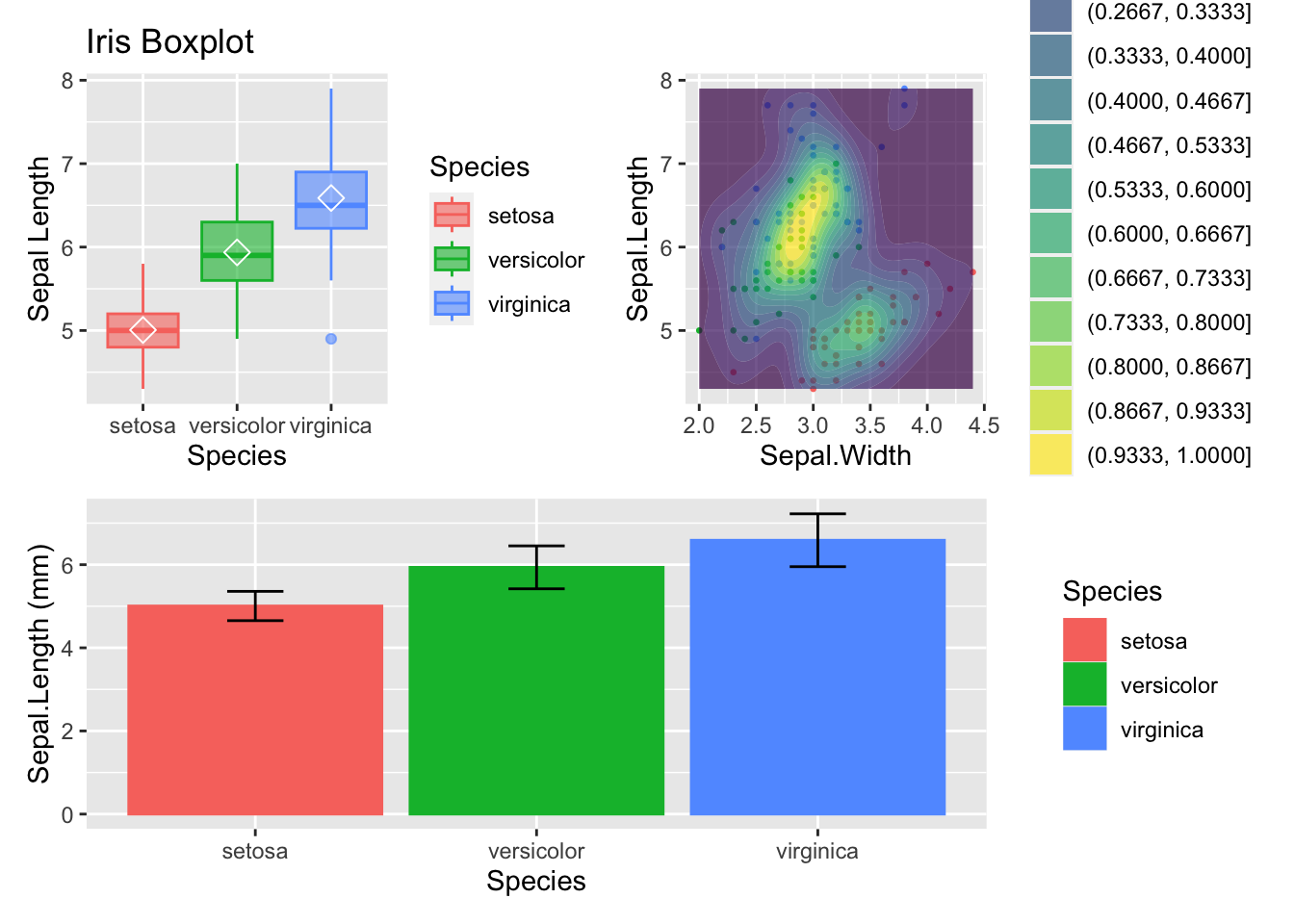
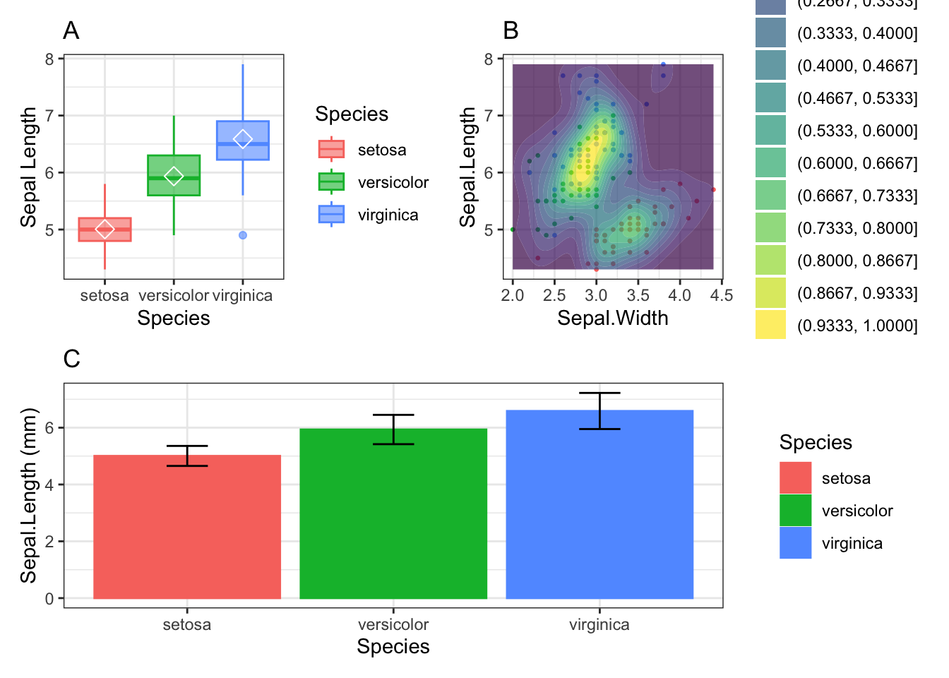
ggplot(data = iris, aes(Sepal.Length, Sepal.Width))+ # scatter plot 
  geom_point()

Line plot

ggplot(data = iris, aes(Sepal.Length, Sepal.Width))+ # scatter plot 
  geom_line()

How to customise plot

Size and shape of the scatter plot

# Change size, color and shape in a scatter plot 
ggplot(data = iris, aes(Sepal.Length, Sepal.Width))+ # scatter plot 
  geom_point(size=3, color ="steelblue", shape=21)  # shape is the same thing wiht classical plot on R

Some examples of customization on plot from iris data set

Change the shape and color : color according to species

# We can calorize and give a shape by month 
ggplot(data = iris, aes(Sepal.Length, Sepal.Width))+ # scatter plot 
  geom_point(aes(color = Species, shape = Species)) # shape is the same thing with classical plot on R

Change the shape and color : gradient of color and shape accroding to species

Be carefull alpha option is for transparency and ranged between 0 and 1

ggplot(data = iris, aes(Sepal.Width,Sepal.Length))+  
geom_point(aes(color = Petal.Width, shape = Species), size = 2,alpha=(0.8))

What kind of conclusion we can give me with this kind of graph?

You can defin your own gradiend with scale_color_gradient()

ggplot(data = iris, aes(Sepal.Width,Sepal.Length))+  
geom_point(aes(color = Petal.Width, shape = Species), size = 2,alpha=(0.8))+
scale_color_gradient(low = "yellow", high = "red")

Custom the color for each species, add them and storage of the plot in a object

# You can change manually color with la fonction scale_color_manual()
ggplot(data = iris, aes(Sepal.Length, Sepal.Width))+ # scatter plot 
 geom_point(aes(color = Species, shape = Species))  +
  scale_color_manual(values = c("#00AFBB", "#E7B800", "#FC4E07"))

#You can store your plot in a variable to print later 
p<-ggplot(data = iris, aes(Sepal.Length, Sepal.Width))+ # scatter plot 
 geom_point(aes(color = Species, shape = Species))  +
  scale_color_manual(values = c("#00AFBB", "#E7B800", "#FC4E07"))+
  theme_minimal()
  

print(p)

What do you see if you play the following command : names(p)?

Change legend position and add title with axis label

#To arrange the graph we can add some label and change the position of the legend
p + theme(legend.position = "top")

p + labs(color = "Species", shape= "Sepcies",
  title = "Sepal Length for each speices",
  subtitle = "is a data frame with 150 cases (rows) and 5 variables",
  x = "Sepal.Length (mm)", y = "Sepal.Width (mm)"
  )

Add a trend curve using stat_smooth()

p2<-ggplot(data = iris, aes(Sepal.Length,Petal.Length))+ # scatter plot 
  geom_point(size=3, color ="steelblue") +
  stat_smooth(method=lm, se=TRUE, na.rm=TRUE, show.legend = TRUE)
p2 + labs(x = "Sepal.Length (mm)", y = "Pepal.Length (mm)")

`geom_smooth()` using formula = 'y ~ x'

To get data from the trend

ggplot_build(p2)$data[[2]]

`geom_smooth()` using formula = 'y ~ x'

          x         y      ymin     ymax         se flipped_aes PANEL group
1  4.300000 0.8898184 0.5928870 1.186750 0.15025965       FALSE     1    -1
2  4.345570 0.9745065 0.6843700 1.264643 0.14682115       FALSE     1    -1
3  4.391139 1.0591946 0.7758049 1.342584 0.14340694       FALSE     1    -1
4  4.436709 1.1438827 0.8671884 1.420577 0.14001881       FALSE     1    -1
5  4.482278 1.2285708 0.9585165 1.498625 0.13665869       FALSE     1    -1
6  4.527848 1.3132589 1.0497850 1.576733 0.13332869       FALSE     1    -1
7  4.573418 1.3979469 1.1409895 1.654904 0.13003114       FALSE     1    -1
8  4.618987 1.4826350 1.2321248 1.733145 0.12676857       FALSE     1    -1
9  4.664557 1.5673231 1.3231856 1.811461 0.12354374       FALSE     1    -1
10 4.710127 1.6520112 1.4141657 1.889857 0.12035969       FALSE     1    -1
11 4.755696 1.7366993 1.5050587 1.968340 0.11721974       FALSE     1    -1
12 4.801266 1.8213874 1.5958574 2.046917 0.11412754       FALSE     1    -1
13 4.846835 1.9060755 1.6865538 2.125597 0.11108706       FALSE     1    -1
14 4.892405 1.9907635 1.7771394 2.204388 0.10810268       FALSE     1    -1
15 4.937975 2.0754516 1.8676047 2.283299 0.10517918       FALSE     1    -1
16 4.983544 2.1601397 1.9579394 2.362340 0.10232176       FALSE     1    -1
17 5.029114 2.2448278 2.0481322 2.441523 0.09953612       FALSE     1    -1
18 5.074684 2.3295159 2.1381710 2.520861 0.09682845       FALSE     1    -1
19 5.120253 2.4142040 2.2280424 2.600366 0.09420548       FALSE     1    -1
20 5.165823 2.4988921 2.3177320 2.680052 0.09167449       FALSE     1    -1
21 5.211392 2.5835801 2.4072245 2.759936 0.08924328       FALSE     1    -1
22 5.256962 2.6682682 2.4965032 2.840033 0.08692025       FALSE     1    -1
23 5.302532 2.7529563 2.5855505 2.920362 0.08471428       FALSE     1    -1
24 5.348101 2.8376444 2.6743480 3.000941 0.08263476       FALSE     1    -1
25 5.393671 2.9223325 2.7628763 3.081789 0.08069145       FALSE     1    -1
26 5.439241 3.0070206 2.8511155 3.162926 0.07889444       FALSE     1    -1
27 5.484810 3.0917086 2.9390454 3.244372 0.07725392       FALSE     1    -1
28 5.530380 3.1763967 3.0266461 3.326147 0.07578006       FALSE     1    -1
29 5.575949 3.2610848 3.1138978 3.408272 0.07448275       FALSE     1    -1
30 5.621519 3.3457729 3.2007821 3.490764 0.07337136       FALSE     1    -1
31 5.667089 3.4304610 3.2872821 3.573640 0.07245446       FALSE     1    -1
32 5.712658 3.5151491 3.3733831 3.656915 0.07173948       FALSE     1    -1
33 5.758228 3.5998372 3.4590730 3.740601 0.07123252       FALSE     1    -1
34 5.803797 3.6845252 3.5443430 3.824707 0.07093803       FALSE     1    -1
35 5.849367 3.7692133 3.6291879 3.909239 0.07085867       FALSE     1    -1
36 5.894937 3.8539014 3.7136063 3.994197 0.07099515       FALSE     1    -1
37 5.940506 3.9385895 3.7976006 4.079578 0.07134624       FALSE     1    -1
38 5.986076 4.0232776 3.8811770 4.165378 0.07190879       FALSE     1    -1
39 6.031646 4.1079657 3.9643453 4.251586 0.07267789       FALSE     1    -1
40 6.077215 4.1926538 4.0471181 4.338189 0.07364708       FALSE     1    -1
41 6.122785 4.2773418 4.1295109 4.425173 0.07480857       FALSE     1    -1
42 6.168354 4.3620299 4.2115411 4.512519 0.07615357       FALSE     1    -1
43 6.213924 4.4467180 4.2932276 4.600208 0.07767254       FALSE     1    -1
44 6.259494 4.5314061 4.3745899 4.688222 0.07935550       FALSE     1    -1
45 6.305063 4.6160942 4.4556484 4.776540 0.08119225       FALSE     1    -1
46 6.350633 4.7007823 4.5364230 4.865141 0.08317259       FALSE     1    -1
47 6.396203 4.7854704 4.6169337 4.954007 0.08528654       FALSE     1    -1
48 6.441772 4.8701584 4.6971995 5.043117 0.08752440       FALSE     1    -1
49 6.487342 4.9548465 4.7772387 5.132454 0.08987692       FALSE     1    -1
50 6.532911 5.0395346 4.8570686 5.222001 0.09233535       FALSE     1    -1
51 6.578481 5.1242227 4.9367056 5.311740 0.09489144       FALSE     1    -1
52 6.624051 5.2089108 5.0161647 5.401657 0.09753752       FALSE     1    -1
53 6.669620 5.2935989 5.0954600 5.491738 0.10026647       FALSE     1    -1
54 6.715190 5.3782869 5.1746046 5.581969 0.10307170       FALSE     1    -1
55 6.760759 5.4629750 5.2536105 5.672340 0.10594715       FALSE     1    -1
56 6.806329 5.5476631 5.3324885 5.762838 0.10888727       FALSE     1    -1
57 6.851899 5.6323512 5.4112489 5.853454 0.11188695       FALSE     1    -1
58 6.897468 5.7170393 5.4899007 5.944178 0.11494153       FALSE     1    -1
59 6.943038 5.8017274 5.5684525 6.035002 0.11804675       FALSE     1    -1
60 6.988608 5.8864155 5.6469119 6.125919 0.12119872       FALSE     1    -1
61 7.034177 5.9711035 5.7252860 6.216921 0.12439388       FALSE     1    -1
62 7.079747 6.0557916 5.8035811 6.308002 0.12762899       FALSE     1    -1
63 7.125316 6.1404797 5.8818031 6.399156 0.13090109       FALSE     1    -1
64 7.170886 6.2251678 5.9599574 6.490378 0.13420747       FALSE     1    -1
65 7.216456 6.3098559 6.0380488 6.581663 0.13754566       FALSE     1    -1
66 7.262025 6.3945440 6.1160818 6.673006 0.14091339       FALSE     1    -1
67 7.307595 6.4792321 6.1940606 6.764404 0.14430861       FALSE     1    -1
68 7.353165 6.5639201 6.2719887 6.855852 0.14772942       FALSE     1    -1
69 7.398734 6.6486082 6.3498697 6.947347 0.15117407       FALSE     1    -1
70 7.444304 6.7332963 6.4277068 7.038886 0.15464098       FALSE     1    -1
71 7.489873 6.8179844 6.5055028 7.130466 0.15812868       FALSE     1    -1
72 7.535443 6.9026725 6.5832603 7.222085 0.16163582       FALSE     1    -1
73 7.581013 6.9873606 6.6609818 7.313739 0.16516118       FALSE     1    -1
74 7.626582 7.0720486 6.7386697 7.405428 0.16870359       FALSE     1    -1
75 7.672152 7.1567367 6.8163259 7.497148 0.17226202       FALSE     1    -1
76 7.717722 7.2414248 6.8939523 7.588897 0.17583549       FALSE     1    -1
77 7.763291 7.3261129 6.9715509 7.680675 0.17942310       FALSE     1    -1
78 7.808861 7.4108010 7.0491231 7.772479 0.18302403       FALSE     1    -1
79 7.854430 7.4954891 7.1266705 7.864308 0.18663749       FALSE     1    -1
80 7.900000 7.5801772 7.2041946 7.956160 0.19026278       FALSE     1    -1
    colour   fill linewidth linetype weight alpha
1  #3366FF grey60         1        1      1   0.4
2  #3366FF grey60         1        1      1   0.4
3  #3366FF grey60         1        1      1   0.4
4  #3366FF grey60         1        1      1   0.4
5  #3366FF grey60         1        1      1   0.4
6  #3366FF grey60         1        1      1   0.4
7  #3366FF grey60         1        1      1   0.4
8  #3366FF grey60         1        1      1   0.4
9  #3366FF grey60         1        1      1   0.4
10 #3366FF grey60         1        1      1   0.4
11 #3366FF grey60         1        1      1   0.4
12 #3366FF grey60         1        1      1   0.4
13 #3366FF grey60         1        1      1   0.4
14 #3366FF grey60         1        1      1   0.4
15 #3366FF grey60         1        1      1   0.4
16 #3366FF grey60         1        1      1   0.4
17 #3366FF grey60         1        1      1   0.4
18 #3366FF grey60         1        1      1   0.4
19 #3366FF grey60         1        1      1   0.4
20 #3366FF grey60         1        1      1   0.4
21 #3366FF grey60         1        1      1   0.4
22 #3366FF grey60         1        1      1   0.4
23 #3366FF grey60         1        1      1   0.4
24 #3366FF grey60         1        1      1   0.4
25 #3366FF grey60         1        1      1   0.4
26 #3366FF grey60         1        1      1   0.4
27 #3366FF grey60         1        1      1   0.4
28 #3366FF grey60         1        1      1   0.4
29 #3366FF grey60         1        1      1   0.4
30 #3366FF grey60         1        1      1   0.4
31 #3366FF grey60         1        1      1   0.4
32 #3366FF grey60         1        1      1   0.4
33 #3366FF grey60         1        1      1   0.4
34 #3366FF grey60         1        1      1   0.4
35 #3366FF grey60         1        1      1   0.4
36 #3366FF grey60         1        1      1   0.4
37 #3366FF grey60         1        1      1   0.4
38 #3366FF grey60         1        1      1   0.4
39 #3366FF grey60         1        1      1   0.4
40 #3366FF grey60         1        1      1   0.4
41 #3366FF grey60         1        1      1   0.4
42 #3366FF grey60         1        1      1   0.4
43 #3366FF grey60         1        1      1   0.4
44 #3366FF grey60         1        1      1   0.4
45 #3366FF grey60         1        1      1   0.4
46 #3366FF grey60         1        1      1   0.4
47 #3366FF grey60         1        1      1   0.4
48 #3366FF grey60         1        1      1   0.4
49 #3366FF grey60         1        1      1   0.4
50 #3366FF grey60         1        1      1   0.4
51 #3366FF grey60         1        1      1   0.4
52 #3366FF grey60         1        1      1   0.4
53 #3366FF grey60         1        1      1   0.4
54 #3366FF grey60         1        1      1   0.4
55 #3366FF grey60         1        1      1   0.4
56 #3366FF grey60         1        1      1   0.4
57 #3366FF grey60         1        1      1   0.4
58 #3366FF grey60         1        1      1   0.4
59 #3366FF grey60         1        1      1   0.4
60 #3366FF grey60         1        1      1   0.4
61 #3366FF grey60         1        1      1   0.4
62 #3366FF grey60         1        1      1   0.4
63 #3366FF grey60         1        1      1   0.4
64 #3366FF grey60         1        1      1   0.4
65 #3366FF grey60         1        1      1   0.4
66 #3366FF grey60         1        1      1   0.4
67 #3366FF grey60         1        1      1   0.4
68 #3366FF grey60         1        1      1   0.4
69 #3366FF grey60         1        1      1   0.4
70 #3366FF grey60         1        1      1   0.4
71 #3366FF grey60         1        1      1   0.4
72 #3366FF grey60         1        1      1   0.4
73 #3366FF grey60         1        1      1   0.4
74 #3366FF grey60         1        1      1   0.4
75 #3366FF grey60         1        1      1   0.4
76 #3366FF grey60         1        1      1   0.4
77 #3366FF grey60         1        1      1   0.4
78 #3366FF grey60         1        1      1   0.4
79 #3366FF grey60         1        1      1   0.4
80 #3366FF grey60         1        1      1   0.4

Density plot

 ggplot(data = iris)+
geom_density(aes(x = Sepal.Length, fill = "Sepal.Length"))

And I add a layer…

ggplot(data = iris)+
geom_density(aes(x = Sepal.Length, fill = "Sepal.Length"))+
geom_density(aes(x = Sepal.Width, fill = "Sepal.Width"))

one more

ggplot(data = iris)+
geom_density(aes(x = Sepal.Length, fill = "Sepal.Length"))+
geom_density(aes(x = Sepal.Width, fill = "Sepal.Width"))+
geom_density(aes(x = Petal.Width, fill = "Petal.Width"))

And the last one with some aesthics

ggplot(data = iris)+
geom_density(aes(x = Sepal.Length, fill = "Sepal.Length"), alpha=0.4,color=NA)+
geom_density(aes(x = Sepal.Width, fill = "Sepal.Width"), alpha=0.4,color=NA)+
geom_density(aes(x = Petal.Width, fill = "Petal.Width"), alpha=0.4,color=NA)+
geom_density(aes(x = Petal.Length, fill = "Petal.Length"), alpha=0.4,color=NA)+
labs(x="cm", y="Fréquence")

Bar plot

my_df<-iris %>%
  group_by(Species)%>%
  summarise(moyenne=mean(Sepal.Length, na.rm=TRUE), sd=sd(Sepal.Length, na.rm=TRUE))

my_df<-as.data.frame(my_df)

ggplot(data = my_df, aes(Species, moyenne))+# scatter plot
  geom_col(aes(color= Species, fill=Species))+
  labs(x="Species", y="Sepal.Length (mm)")+
  geom_errorbar(aes(ymin = moyenne-sd, ymax = moyenne+sd), width=0.2)

Boxplot

ggplot(data = iris, aes(Species, Sepal.Length))+ 
  geom_boxplot()+
  labs(x="Species", y="Sepal.Length (mm)")+
  theme_minimal()

With some aesthetics : color by species, transparency and theme

ggplot(data = iris, aes(Species, Sepal.Length))+
  geom_boxplot(aes(color=Species, fill=Species), alpha=0.4)+
  labs(x="Species", y="Sepal.Length (mm)")+
  theme_minimal()

I add data on the boxplot

ggplot(data = iris, aes(Species, Sepal.Length))+
  geom_boxplot(aes(color=Species, fill=Species), alpha=0.4)+
  geom_jitter(aes(colour = Species), position = position_jitter(0.07), cex = 2.2)+
  labs(x="Species", y="Sepal.Length (mm)")+
  theme_minimal()

Or I add mean on boxplot

ggplot(data=iris, aes(x=Species, y=Sepal.Length))+
geom_boxplot(aes(fill=Species,col=Species),alpha=0.6)+
labs(x="Species",y="Sepal Length", title="Iris Boxplot")+
stat_summary(fun=mean, geom="point", shape=5, col="white", size=3)

2D approach: geom_density2d

Note density throughout contour lines

ggplot(data=iris,aes(x=Sepal.Width,y=Sepal.Length, color=Species))+ 
geom_density2d()

I plot data on the contour plot

ggplot(data=iris,aes(x=Sepal.Width,y=Sepal.Length, color=Species)) +
geom_point()+
geom_density2d()

Color areas/density band : geom_density_2d_filled

Density across “bands”. Note:contour_var = “ndensity”: Normalise intensity to 1.

ggplot(data=iris,aes(x=Sepal.Width,y=Sepal.Length)) +
geom_point(cex=0.8)+
geom_density_2d_filled(alpha = 0.5,bins=5,contour_var = "ndensity")

ggplot(data=iris,aes(x=Sepal.Width,y=Sepal.Length)) +
geom_point(aes(col=Species),cex=0.5)+
geom_density_2d_filled(alpha = 0.7,contour_var = "ndensity", bins=15)

Save your plot

pdf("yourfile.pdf")
ggplot(data = iris, aes(Species, Sepal.Length))+
  geom_boxplot(aes(color=Species, fill=Species), alpha=0.4)+
  geom_jitter(aes(colour = Species), position = position_jitter(0.07), cex = 2.2)+
  labs(x="Species", y="Sepal.Length (mm)")+
  theme_minimal()
dev.off()

quartz_off_screen 
                2

How to make a figure with different pannel?

For this, we will use facet_wrap option on iris data

ggplot(data = iris, aes(Sepal.Length,Petal.Length))+
  geom_point(aes(shape = Species))+
  facet_wrap(~Species, scales = "free")

Note

Library patchwork offers more adventage to custom your different panel. You can find here more information about patchwork packages

library(patchwork)
g1<-ggplot(data=iris, aes(x=Species, y=Sepal.Length))+
geom_boxplot(aes(fill=Species,col=Species),alpha=0.6)+
labs(x="Species",y="Sepal Length", title="Iris Boxplot")+
stat_summary(fun=mean, geom="point", shape=5, col="white", size=3) 

g2<-ggplot(data=iris,aes(x=Sepal.Width,y=Sepal.Length)) +
geom_point(aes(col=Species),cex=0.5)+
geom_density_2d_filled(alpha = 0.7,contour_var = "ndensity", bins=15)

g3<-ggplot(data = my_df, aes(Species, moyenne))+# scatter plot
  geom_col(aes(color= Species, fill=Species))+
  labs(x="Species", y="Sepal.Length (mm)")+
  geom_errorbar(aes(ymin = moyenne-sd, ymax = moyenne+sd), width=0.2)

(g1|g2)/g3

library(patchwork)
g1<-ggplot(data=iris, aes(x=Species, y=Sepal.Length))+
  geom_boxplot(aes(fill=Species,col=Species),alpha=0.6)+
  labs(x="Species",y="Sepal Length", title="Iris Boxplot")+
  stat_summary(fun=mean, geom="point", shape=5, col="white", size=3)+
  theme_bw()+
  ggtitle("A")

g2<-ggplot(data=iris,aes(x=Sepal.Width,y=Sepal.Length)) +
  geom_point(aes(col=Species),cex=0.5)+
  geom_density_2d_filled(alpha = 0.7,contour_var = "ndensity", bins=15)+
  theme_bw()+
  ggtitle("B")

g3<-ggplot(data = my_df, aes(Species, moyenne))+# scatter plot
  geom_col(aes(color= Species, fill=Species))+
  labs(x="Species", y="Sepal.Length (mm)")+
  geom_errorbar(aes(ymin = moyenne-sd, ymax = moyenne+sd), width=0.2)+
  theme_bw()+
  ggtitle("C")

(g1|g2)/g3

Interactive graph using plotly package

If not installed, you have to install it and load it

p4<-ggplot(data = iris, aes(Species, Sepal.Length))+
  geom_boxplot(aes(color=Species, fill=Species), alpha=0.4)+
  geom_jitter(aes(colour = Species), position = position_jitter(0.07), cex = 2.2)+
  labs(x="Species", y="Sepal.Length (mm)")+
  theme_minimal()

plotly::ggplotly(p4, height = 350, width=800)

Exo 1

Read the data set mapfileFa.txt
Give me the structure of the data set, and explore the data set. Dimension of the data set ? What kind of variable do you have?
Give me the distribution Chlorophyl and Nanoeukaryote using ggplot and geom_boxplot() colored by the geography. Using the package patchwork build figure with these two plots on a same pages and save it as pdf
Add a variable into the data frame as the ratio between NT and PT. Build a scatter of the ratio NT/PT as a function sample name and sort by geography using facet_wrap function. Change x and y label as Sample Name and Ratio NR/TP. Give a title at your figure.
Group dataset by the geography and calculate the mean and the sd of the number of Crypto. Build a bar plot with mean and error bar (sd) colored according to the geography.
Save figure as pdf
Filter South data in a new data frame. Build a scatter plot, with size of shape = 3 and color = red. Add a trend curve.
Do the the same for northern site.