Statistics

Author

Marc Garel & Fabrice Armougom

Load libraries & functions

#libraries
library(ggplot2)
library(base)
library(psych)
library(dplyr)
library(stats)
library(FSA)
library(ggpubr)
library(corrplot)
library(ggpmisc)
library(graphics)
library(broom)
library(tidyr)

#Function indice_normality
indices_normality <- function(rich, nrow, ncol) {

  ### p-value < 0.05 means data failed normality test

  par(mfrow = c(nrow, ncol))

  for (i in names(rich)) {
    shap <- shapiro.test(rich[, i])
    qqnorm(rich[, i], main = i, sub = shap$p.value)
    qqline(rich[, i])
  }

  par(mfrow = c(1, 1))
}
############
#Function multiple panel with linear regression & r values
regression_line = function(x,y, ...){
    points(x,y,...)
    linear_regression = lm(y~x)
    linear_regression_line = abline(linear_regression, col="red")
}
###########
panel.cor <- function(x, y, digits = 2, prefix = "", cex.cor, ...) {
  usr <- par("usr")
  on.exit(par(usr))
  par(usr = c(0, 1, 0, 1))
  r <- abs(cor(x, y, use = "complete.obs"))
  txt <- format(c(r, 0.123456789), digits = digits)[1]
  txt <- paste(prefix, txt, sep = "")
  if (missing(cex.cor)) cex.cor <- 0.8/strwidth(txt)
  text(0.5, 0.5, txt, cex =  cex.cor * (1 + r) / 2)
}

I- Manipulate a data table

a/ Read a table containing data

alldata = read.table(file ="./data/data_explore.txt",
                      check.names = TRUE,
                      header = TRUE, 
                      sep = "\t",
                      row.names = 1)

#see
alldata

    Description Geo groupe SiOH4   NO2   NO3   NH4   PO4    NT    PT  Chla
U1H       USA_H USA      A  1690 2.324 0.083 0.856 0.467 0.115 9.539 4.138
U2H       USA_H USA      A   115 1.813 0.256 0.889 0.324 0.132 9.946 3.565
U3H       USA_H USA      A   395 2.592 0.105 1.125 0.328 0.067 9.378 3.391
U4H       USA_H USA      A   395 2.381 0.231 0.706 0.450 0.109 8.817 3.345
U5F       USA_F USA      B   200 1.656 0.098 0.794 0.367 0.095 7.847 2.520
U6F       USA_F USA      B   235 2.457 0.099 1.087 0.349 0.137 8.689 3.129
U7F       USA_F USA      B   235 2.457 0.099 1.087 0.349 0.137 8.689 3.129
U8F       USA_F USA      B  1355 2.028 0.103 1.135 0.216 0.128 8.623 3.137
E1H        EU_H  EU      C   945 2.669 0.136 0.785 0.267 0.114 9.146 3.062
E2H        EU_H  EU      C  1295 2.206 0.249 0.768 0.629 0.236 9.013 3.455
E3H        EU_H  EU      C  1300 3.004 0.251 0.727 0.653 0.266 8.776 3.230
E4H        EU_H  EU      C  1600 3.016 0.257 0.695 0.491 0.176 8.968 4.116
E5F        EU_F  EU      D  1355 1.198 0.165 1.099 0.432 0.180 8.256 3.182
E6F        EU_F  EU      D  1590 3.868 0.253 0.567 0.533 0.169 8.395 3.126
E7F        EU_F  EU      D  2265 3.639 0.255 0.658 0.665 0.247 8.991 3.843
E8F        EU_F  EU      D  1180 3.910 0.107 0.472 0.490 0.134 8.954 4.042
E9F        EU_F  EU      D  1545 3.607 0.139 0.444 0.373 0.167 9.817 3.689
         T       S Sigma_t observed   shannon evenness dominance_relative
U1H 0.0182 23.0308 38.9967  26.9631 0.9447863 3.146480          0.8780420
U2H 0.0000 22.7338 37.6204  26.0046 0.9477924 3.177766          0.8937989
U3H 0.0000 22.6824 37.6627  26.0521 0.9577758 3.408022          0.9060997
U4H 0.0000 22.6854 37.6176  26.0137 0.9414576 3.112066          0.8684385
U5F 0.0000 22.5610 37.5960  26.0332 0.9491313 3.246802          0.8925706
U6F 0.0000 18.8515 37.4542  26.9415 0.9570249 3.350694          0.9083230
U7F 0.0000 18.8515 37.4542  26.9415 0.9363446 3.097474          0.8396788
U8F 0.0102 24.1905 38.3192  26.1037 0.9271578 2.978541          0.8594252
E1H 0.0000 24.1789 38.3213  26.1065 0.9253250 2.993341          0.8560944
E2H 0.0000 22.0197 39.0877  27.3241 0.9439556 3.213508          0.8653415
E3H 0.0134 22.0515 39.0884  27.3151 0.8247810 2.440971          0.7325395
E4H 0.0000 23.6669 38.9699  26.7536 0.9435901 3.157702          0.8811735
E5F 0.0000 23.6814 38.9708  26.7488 0.9488744 3.278296          0.8663140
E6F 0.0000 23.1236 39.0054  26.9423 0.9452117 3.108474          0.8890226
E7F 0.0132 23.3147 38.9885  26.8713 0.9517578 3.307644          0.9028494
E8F 0.0172 22.6306 38.9094  27.0131 0.9443038 3.105908          0.8667202
E9F 0.0062 22.9545 38.7777  26.8172 0.9487545 3.180393          0.9095912
           NRI         NTI          PD        X
U1H 0.10274791 -1.72903786 -1.62669669 3.508045
U2H 0.10274791  1.12496864 -0.75543498 3.330466
U3H 0.09677419 -0.23029299 -0.69141166 3.688595
U4H 0.10991637 -2.48017258 -0.64705490 3.401944
U5F 0.10991637 -0.17940416 -0.67857965 3.430623
U6F 0.08721625 -0.40633803  0.05055793 3.293266
U7F 0.14336918  1.79668405 -0.84513858 3.428512
U8F 0.16606930  0.12915148  0.12211753 2.969649
E1H 0.18876941 -0.07458097  1.95798975 2.451799
E2H 0.13620072  0.17114822  1.11902329 3.127781
E3H 0.38351254  2.65479470 -0.01038346 2.422910
E4H 0.13022700 -1.42798211 -0.64181960 3.157211
E5F 0.10633214 -2.49590494  0.79285403 3.433528
E6F 0.09438471 -0.10962187  0.81104335 2.921706
E7F 0.09677419 -1.21112926  0.51096388 3.282069
E8F 0.09438471 -0.04833770  0.26352612 2.879671
E9F 0.10394265  0.50404786  2.43432750 2.430342

1- Can you display only the column NO3 of the table?

2- Can you display the row names of the table? (means U1H, U2H etc)

3- Can you select and display any 3 columns of the table?

b/ Select a subset from data table

#Keep only data that correspond to "EU" in the Geo column
subgroupEU = subset(alldata, Geo=="EU")
#See 
subgroupEU

    Description Geo groupe SiOH4   NO2   NO3   NH4   PO4    NT    PT  Chla
E1H        EU_H  EU      C   945 2.669 0.136 0.785 0.267 0.114 9.146 3.062
E2H        EU_H  EU      C  1295 2.206 0.249 0.768 0.629 0.236 9.013 3.455
E3H        EU_H  EU      C  1300 3.004 0.251 0.727 0.653 0.266 8.776 3.230
E4H        EU_H  EU      C  1600 3.016 0.257 0.695 0.491 0.176 8.968 4.116
E5F        EU_F  EU      D  1355 1.198 0.165 1.099 0.432 0.180 8.256 3.182
E6F        EU_F  EU      D  1590 3.868 0.253 0.567 0.533 0.169 8.395 3.126
E7F        EU_F  EU      D  2265 3.639 0.255 0.658 0.665 0.247 8.991 3.843
E8F        EU_F  EU      D  1180 3.910 0.107 0.472 0.490 0.134 8.954 4.042
E9F        EU_F  EU      D  1545 3.607 0.139 0.444 0.373 0.167 9.817 3.689
         T       S Sigma_t observed   shannon evenness dominance_relative
E1H 0.0000 24.1789 38.3213  26.1065 0.9253250 2.993341          0.8560944
E2H 0.0000 22.0197 39.0877  27.3241 0.9439556 3.213508          0.8653415
E3H 0.0134 22.0515 39.0884  27.3151 0.8247810 2.440971          0.7325395
E4H 0.0000 23.6669 38.9699  26.7536 0.9435901 3.157702          0.8811735
E5F 0.0000 23.6814 38.9708  26.7488 0.9488744 3.278296          0.8663140
E6F 0.0000 23.1236 39.0054  26.9423 0.9452117 3.108474          0.8890226
E7F 0.0132 23.3147 38.9885  26.8713 0.9517578 3.307644          0.9028494
E8F 0.0172 22.6306 38.9094  27.0131 0.9443038 3.105908          0.8667202
E9F 0.0062 22.9545 38.7777  26.8172 0.9487545 3.180393          0.9095912
           NRI         NTI          PD        X
E1H 0.18876941 -0.07458097  1.95798975 2.451799
E2H 0.13620072  0.17114822  1.11902329 3.127781
E3H 0.38351254  2.65479470 -0.01038346 2.422910
E4H 0.13022700 -1.42798211 -0.64181960 3.157211
E5F 0.10633214 -2.49590494  0.79285403 3.433528
E6F 0.09438471 -0.10962187  0.81104335 2.921706
E7F 0.09677419 -1.21112926  0.51096388 3.282069
E8F 0.09438471 -0.04833770  0.26352612 2.879671
E9F 0.10394265  0.50404786  2.43432750 2.430342

#Keep only data that correspond to group A & B in the group column
subgroupAB = subset(alldata, groupe=="A" | groupe=="B")
#See
subgroupAB

    Description Geo groupe SiOH4   NO2   NO3   NH4   PO4    NT    PT  Chla
U1H       USA_H USA      A  1690 2.324 0.083 0.856 0.467 0.115 9.539 4.138
U2H       USA_H USA      A   115 1.813 0.256 0.889 0.324 0.132 9.946 3.565
U3H       USA_H USA      A   395 2.592 0.105 1.125 0.328 0.067 9.378 3.391
U4H       USA_H USA      A   395 2.381 0.231 0.706 0.450 0.109 8.817 3.345
U5F       USA_F USA      B   200 1.656 0.098 0.794 0.367 0.095 7.847 2.520
U6F       USA_F USA      B   235 2.457 0.099 1.087 0.349 0.137 8.689 3.129
U7F       USA_F USA      B   235 2.457 0.099 1.087 0.349 0.137 8.689 3.129
U8F       USA_F USA      B  1355 2.028 0.103 1.135 0.216 0.128 8.623 3.137
         T       S Sigma_t observed   shannon evenness dominance_relative
U1H 0.0182 23.0308 38.9967  26.9631 0.9447863 3.146480          0.8780420
U2H 0.0000 22.7338 37.6204  26.0046 0.9477924 3.177766          0.8937989
U3H 0.0000 22.6824 37.6627  26.0521 0.9577758 3.408022          0.9060997
U4H 0.0000 22.6854 37.6176  26.0137 0.9414576 3.112066          0.8684385
U5F 0.0000 22.5610 37.5960  26.0332 0.9491313 3.246802          0.8925706
U6F 0.0000 18.8515 37.4542  26.9415 0.9570249 3.350694          0.9083230
U7F 0.0000 18.8515 37.4542  26.9415 0.9363446 3.097474          0.8396788
U8F 0.0102 24.1905 38.3192  26.1037 0.9271578 2.978541          0.8594252
           NRI        NTI          PD        X
U1H 0.10274791 -1.7290379 -1.62669669 3.508045
U2H 0.10274791  1.1249686 -0.75543498 3.330466
U3H 0.09677419 -0.2302930 -0.69141166 3.688595
U4H 0.10991637 -2.4801726 -0.64705490 3.401944
U5F 0.10991637 -0.1794042 -0.67857965 3.430623
U6F 0.08721625 -0.4063380  0.05055793 3.293266
U7F 0.14336918  1.7966841 -0.84513858 3.428512
U8F 0.16606930  0.1291515  0.12211753 2.969649

c/ How to Add a new variable after loading table
You forgot to add a variable to your table & you have already loaded your table in R session…how to manage this?

# FIRST create a dataframe with a vector with  values of your new variable
mydataframe = data.frame(MYNEWVAR = c("sediment", "mer", "sediment",
                                       "trap", "mer", "mer",
                                       "trap", "trap", "trap",
                                       "sediment", "mer", "mer",
                                       "mer", "trap", "trap",
                                       "mer", "mer"))

#Add rownames=samples names
row.names(mydataframe) = c("U1H", "U2H", "U5F",
                            "U6F", "U3H", "U7F",
                            "U4H", "U8F", "E2H",
                            "E3H", "E5F", "E1H",
                            "E7F", "E6F", "E4H",
                            "E9F", "E8F")

# See & notice that order of sample names is not the same as in mesdata
mydataframe

    MYNEWVAR
U1H sediment
U2H      mer
U5F sediment
U6F     trap
U3H      mer
U7F      mer
U4H     trap
U8F     trap
E2H     trap
E3H sediment
E5F      mer
E1H      mer
E7F      mer
E6F     trap
E4H     trap
E9F      mer
E8F      mer

Merge the two dataframes!

#Option "by=" the way that you want to merge... here looking for same row.names between the two dataframe
# in mydataframe and mesdata
alldata = merge(alldata,mydataframe, by="row.names")

#check that it works
alldata

   Row.names Description Geo groupe SiOH4   NO2   NO3   NH4   PO4    NT    PT
1        E1H        EU_H  EU      C   945 2.669 0.136 0.785 0.267 0.114 9.146
2        E2H        EU_H  EU      C  1295 2.206 0.249 0.768 0.629 0.236 9.013
3        E3H        EU_H  EU      C  1300 3.004 0.251 0.727 0.653 0.266 8.776
4        E4H        EU_H  EU      C  1600 3.016 0.257 0.695 0.491 0.176 8.968
5        E5F        EU_F  EU      D  1355 1.198 0.165 1.099 0.432 0.180 8.256
6        E6F        EU_F  EU      D  1590 3.868 0.253 0.567 0.533 0.169 8.395
7        E7F        EU_F  EU      D  2265 3.639 0.255 0.658 0.665 0.247 8.991
8        E8F        EU_F  EU      D  1180 3.910 0.107 0.472 0.490 0.134 8.954
9        E9F        EU_F  EU      D  1545 3.607 0.139 0.444 0.373 0.167 9.817
10       U1H       USA_H USA      A  1690 2.324 0.083 0.856 0.467 0.115 9.539
11       U2H       USA_H USA      A   115 1.813 0.256 0.889 0.324 0.132 9.946
12       U3H       USA_H USA      A   395 2.592 0.105 1.125 0.328 0.067 9.378
13       U4H       USA_H USA      A   395 2.381 0.231 0.706 0.450 0.109 8.817
14       U5F       USA_F USA      B   200 1.656 0.098 0.794 0.367 0.095 7.847
15       U6F       USA_F USA      B   235 2.457 0.099 1.087 0.349 0.137 8.689
16       U7F       USA_F USA      B   235 2.457 0.099 1.087 0.349 0.137 8.689
17       U8F       USA_F USA      B  1355 2.028 0.103 1.135 0.216 0.128 8.623
    Chla      T       S Sigma_t observed   shannon evenness dominance_relative
1  3.062 0.0000 24.1789 38.3213  26.1065 0.9253250 2.993341          0.8560944
2  3.455 0.0000 22.0197 39.0877  27.3241 0.9439556 3.213508          0.8653415
3  3.230 0.0134 22.0515 39.0884  27.3151 0.8247810 2.440971          0.7325395
4  4.116 0.0000 23.6669 38.9699  26.7536 0.9435901 3.157702          0.8811735
5  3.182 0.0000 23.6814 38.9708  26.7488 0.9488744 3.278296          0.8663140
6  3.126 0.0000 23.1236 39.0054  26.9423 0.9452117 3.108474          0.8890226
7  3.843 0.0132 23.3147 38.9885  26.8713 0.9517578 3.307644          0.9028494
8  4.042 0.0172 22.6306 38.9094  27.0131 0.9443038 3.105908          0.8667202
9  3.689 0.0062 22.9545 38.7777  26.8172 0.9487545 3.180393          0.9095912
10 4.138 0.0182 23.0308 38.9967  26.9631 0.9447863 3.146480          0.8780420
11 3.565 0.0000 22.7338 37.6204  26.0046 0.9477924 3.177766          0.8937989
12 3.391 0.0000 22.6824 37.6627  26.0521 0.9577758 3.408022          0.9060997
13 3.345 0.0000 22.6854 37.6176  26.0137 0.9414576 3.112066          0.8684385
14 2.520 0.0000 22.5610 37.5960  26.0332 0.9491313 3.246802          0.8925706
15 3.129 0.0000 18.8515 37.4542  26.9415 0.9570249 3.350694          0.9083230
16 3.129 0.0000 18.8515 37.4542  26.9415 0.9363446 3.097474          0.8396788
17 3.137 0.0102 24.1905 38.3192  26.1037 0.9271578 2.978541          0.8594252
          NRI         NTI          PD        X MYNEWVAR
1  0.18876941 -0.07458097  1.95798975 2.451799      mer
2  0.13620072  0.17114822  1.11902329 3.127781     trap
3  0.38351254  2.65479470 -0.01038346 2.422910 sediment
4  0.13022700 -1.42798211 -0.64181960 3.157211     trap
5  0.10633214 -2.49590494  0.79285403 3.433528      mer
6  0.09438471 -0.10962187  0.81104335 2.921706     trap
7  0.09677419 -1.21112926  0.51096388 3.282069      mer
8  0.09438471 -0.04833770  0.26352612 2.879671      mer
9  0.10394265  0.50404786  2.43432750 2.430342      mer
10 0.10274791 -1.72903786 -1.62669669 3.508045 sediment
11 0.10274791  1.12496864 -0.75543498 3.330466      mer
12 0.09677419 -0.23029299 -0.69141166 3.688595      mer
13 0.10991637 -2.48017258 -0.64705490 3.401944     trap
14 0.10991637 -0.17940416 -0.67857965 3.430623 sediment
15 0.08721625 -0.40633803  0.05055793 3.293266     trap
16 0.14336918  1.79668405 -0.84513858 3.428512      mer
17 0.16606930  0.12915148  0.12211753 2.969649     trap

II- Descriptive statistics

Investigates each variable separately. Distribution of individual variables, mean, dispersion

a/ Get stats info for all variables

descriptstats = describe(alldata)
#see
descriptstats

                   vars  n    mean     sd  median trimmed    mad    min     max
Row.names*            1 17    9.00   5.05    9.00    9.00   5.93   1.00   17.00
Description*          2 17    2.41   1.18    2.00    2.40   1.48   1.00    4.00
Geo*                  3 17    1.47   0.51    1.00    1.47   0.00   1.00    2.00
groupe*               4 17    2.59   1.18    3.00    2.60   1.48   1.00    4.00
SiOH4                 5 17 1040.88 653.99 1295.00 1021.00 518.91 115.00 2265.00
NO2                   6 17    2.64   0.78    2.46    2.65   0.81   1.20    3.91
NO3                   7 17    0.17   0.07    0.14    0.17   0.06   0.08    0.26
NH4                   8 17    0.82   0.23    0.78    0.82   0.19   0.44    1.14
PO4                   9 17    0.43   0.13    0.43    0.43   0.12   0.22    0.66
NT                   10 17    0.15   0.05    0.14    0.15   0.04   0.07    0.27
PT                   11 17    8.93   0.54    8.95    8.94   0.39   7.85    9.95
Chla                 12 17    3.42   0.44    3.35    3.43   0.32   2.52    4.14
T                    13 17    0.00   0.01    0.00    0.00   0.00   0.00    0.02
S                    14 17   22.54   1.52   22.73   22.68   0.86  18.85   24.19
Sigma_t              15 17   38.40   0.67   38.78   38.42   0.46  37.45   39.09
observed             16 17   26.64   0.48   26.82   26.64   0.29  26.00   27.32
shannon              17 17    0.94   0.03    0.94    0.94   0.01   0.82    0.96
evenness             18 17    3.14   0.21    3.16    3.16   0.09   2.44    3.41
dominance_relative   19 17    0.87   0.04    0.88    0.88   0.02   0.73    0.91
NRI                  20 17    0.13   0.07    0.11    0.12   0.02   0.09    0.38
NTI                  21 17   -0.24   1.37   -0.11   -0.28   0.91  -2.50    2.65
PD                   22 17    0.13   1.06    0.05    0.09   1.10  -1.63    2.43
X                    23 17    3.13   0.39    3.28    3.14   0.23   2.42    3.69
MYNEWVAR*            24 17    1.88   0.93    2.00    1.87   1.48   1.00    3.00
                     range  skew kurtosis     se
Row.names*           16.00  0.00    -1.41   1.22
Description*          3.00  0.09    -1.59   0.29
Geo*                  1.00  0.11    -2.10   0.12
groupe*               3.00 -0.09    -1.59   0.29
SiOH4              2150.00 -0.06    -1.35 158.62
NO2                   2.71  0.13    -1.03   0.19
NO3                   0.17  0.18    -1.91   0.02
NH4                   0.69  0.03    -1.30   0.05
PO4                   0.45  0.31    -1.03   0.03
NT                    0.20  0.63    -0.62   0.01
PT                    2.10  0.10    -0.49   0.13
Chla                  1.62  0.12    -0.72   0.11
T                     0.02  0.88    -1.01   0.00
S                     5.34 -1.47     1.25   0.37
Sigma_t               1.63 -0.34    -1.81   0.16
observed              1.32 -0.25    -1.60   0.12
shannon               0.13 -2.98     8.28   0.01
evenness              0.97 -1.84     3.97   0.05
dominance_relative    0.18 -2.12     4.77   0.01
NRI                   0.30  2.63     6.58   0.02
NTI                   5.15  0.16    -0.50   0.33
PD                    4.06  0.54    -0.53   0.26
X                     1.27 -0.65    -0.91   0.10
MYNEWVAR*             2.00  0.21    -1.87   0.22

b/ Get stats info by groups

descriptstats_groups = describeBy(alldata, alldata$Geo, skew=FALSE,ranges=FALSE)
#see
descriptstats_groups


 Descriptive statistics by group 
group: EU
                   vars n    mean     sd     se
Row.names*            1 9    5.00   2.74   0.91
Description*          2 9    1.44   0.53   0.18
Geo*                  3 9    1.00   0.00   0.00
groupe*               4 9    3.56   0.53   0.18
SiOH4                 5 9 1452.78 370.60 123.53
NO2                   6 9    3.01   0.89   0.30
NO3                   7 9    0.20   0.06   0.02
NH4                   8 9    0.69   0.20   0.07
PO4                   9 9    0.50   0.13   0.04
NT                   10 9    0.19   0.05   0.02
PT                   11 9    8.92   0.45   0.15
Chla                 12 9    3.53   0.41   0.14
T                    13 9    0.01   0.01   0.00
S                    14 9   23.07   0.74   0.25
Sigma_t              15 9   38.90   0.24   0.08
observed             16 9   26.88   0.36   0.12
shannon              17 9    0.93   0.04   0.01
evenness             18 9    3.09   0.26   0.09
dominance_relative   19 9    0.86   0.05   0.02
NRI                  20 9    0.15   0.09   0.03
NTI                  21 9   -0.23   1.44   0.48
PD                   22 9    0.80   0.95   0.32
X                    23 9    2.90   0.39   0.13
MYNEWVAR*            24 9    1.78   0.97   0.32
------------------------------------------------------------ 
group: USA
                   vars n   mean     sd     se
Row.names*            1 8  13.50   2.45   0.87
Description*          2 8   3.50   0.53   0.19
Geo*                  3 8   2.00   0.00   0.00
groupe*               4 8   1.50   0.53   0.19
SiOH4                 5 8 577.50 597.59 211.28
NO2                   6 8   2.21   0.34   0.12
NO3                   7 8   0.13   0.07   0.02
NH4                   8 8   0.96   0.17   0.06
PO4                   9 8   0.36   0.08   0.03
NT                   10 8   0.12   0.02   0.01
PT                   11 8   8.94   0.65   0.23
Chla                 12 8   3.29   0.46   0.16
T                    13 8   0.00   0.01   0.00
S                    14 8  21.95   1.98   0.70
Sigma_t              15 8  37.84   0.54   0.19
observed             16 8  26.38   0.47   0.17
shannon              17 8   0.95   0.01   0.00
evenness             18 8   3.19   0.14   0.05
dominance_relative   19 8   0.88   0.02   0.01
NRI                  20 8   0.11   0.03   0.01
NTI                  21 8  -0.25   1.38   0.49
PD                   22 8  -0.63   0.55   0.19
X                    23 8   3.38   0.21   0.07
MYNEWVAR*            24 8   2.00   0.93   0.33

c/ Distribution plot

#Distribution of NO2 for all data  
ggplot(data=alldata, aes(x=NO2)) +
geom_density(adjust=1.5, alpha=.4,show.legend=TRUE, fill="red")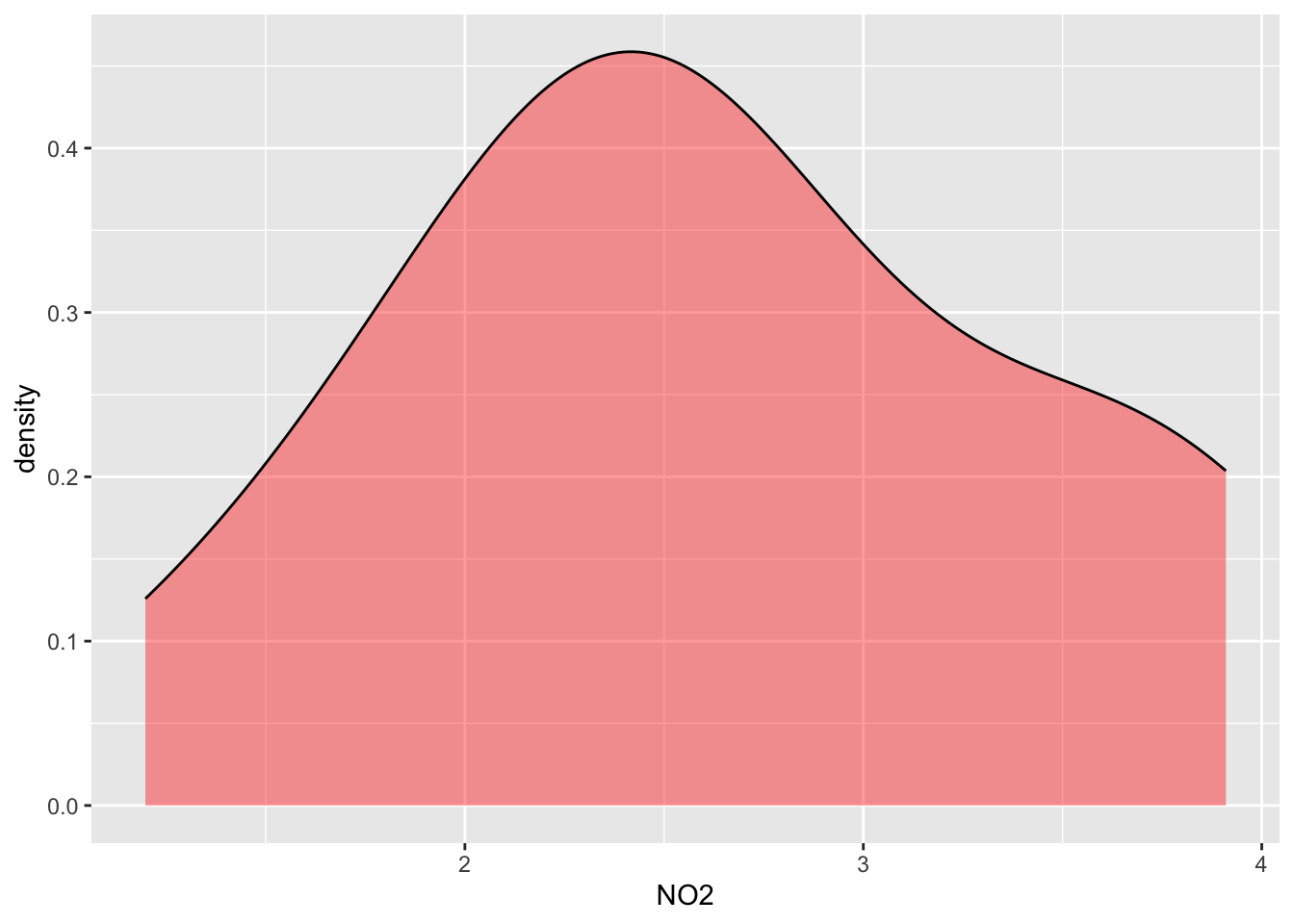

#Distribution of NO2 separated by groups
ggplot(data=alldata, aes(x=NO2, group=Geo, fill=Geo)) +
geom_density(adjust=1.5, alpha=.4)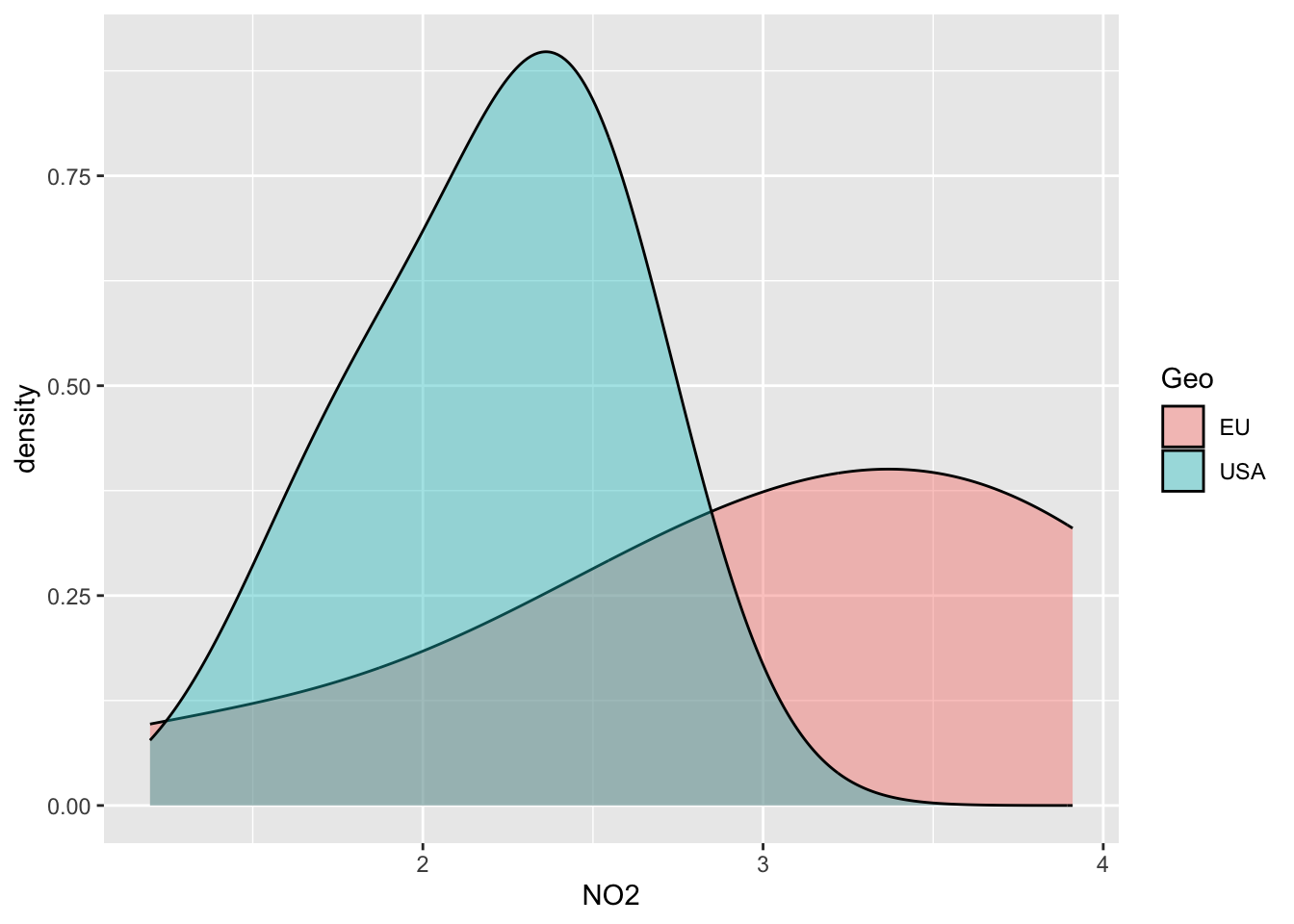

III- Inferential Statistics & Tests

_____________________________________________________________________

Normality test: Check the Normal or not normal distribution of your data to choose the right statistical test!

- Shapiro test: H0 Null Hypothesis: follows Normal distribution!
Means if p<0.05 -> reject the H0 (so does not follow a normal distribution)

- Q-Qplots: Compare your distribution with a theoretical normal distribution
If your data follow a normal distribution, you’re expecting a linear relationship
theoritical vs. experimental
Function indices_normality() plots the results

_____________________________________________________________________

a/ Select indices to test & run normality check : select function

myselection = select(alldata, observed,NRI, evenness)
#See
myselection

   observed        NRI evenness
1   26.1065 0.18876941 2.993341
2   27.3241 0.13620072 3.213508
3   27.3151 0.38351254 2.440971
4   26.7536 0.13022700 3.157702
5   26.7488 0.10633214 3.278296
6   26.9423 0.09438471 3.108474
7   26.8713 0.09677419 3.307644
8   27.0131 0.09438471 3.105908
9   26.8172 0.10394265 3.180393
10  26.9631 0.10274791 3.146480
11  26.0046 0.10274791 3.177766
12  26.0521 0.09677419 3.408022
13  26.0137 0.10991637 3.112066
14  26.0332 0.10991637 3.246802
15  26.9415 0.08721625 3.350694
16  26.9415 0.14336918 3.097474
17  26.1037 0.16606930 2.978541

b/ Run Normality test: QQ-plot +Shapiro

indices_normality(myselection, nrow =3, ncol = 2)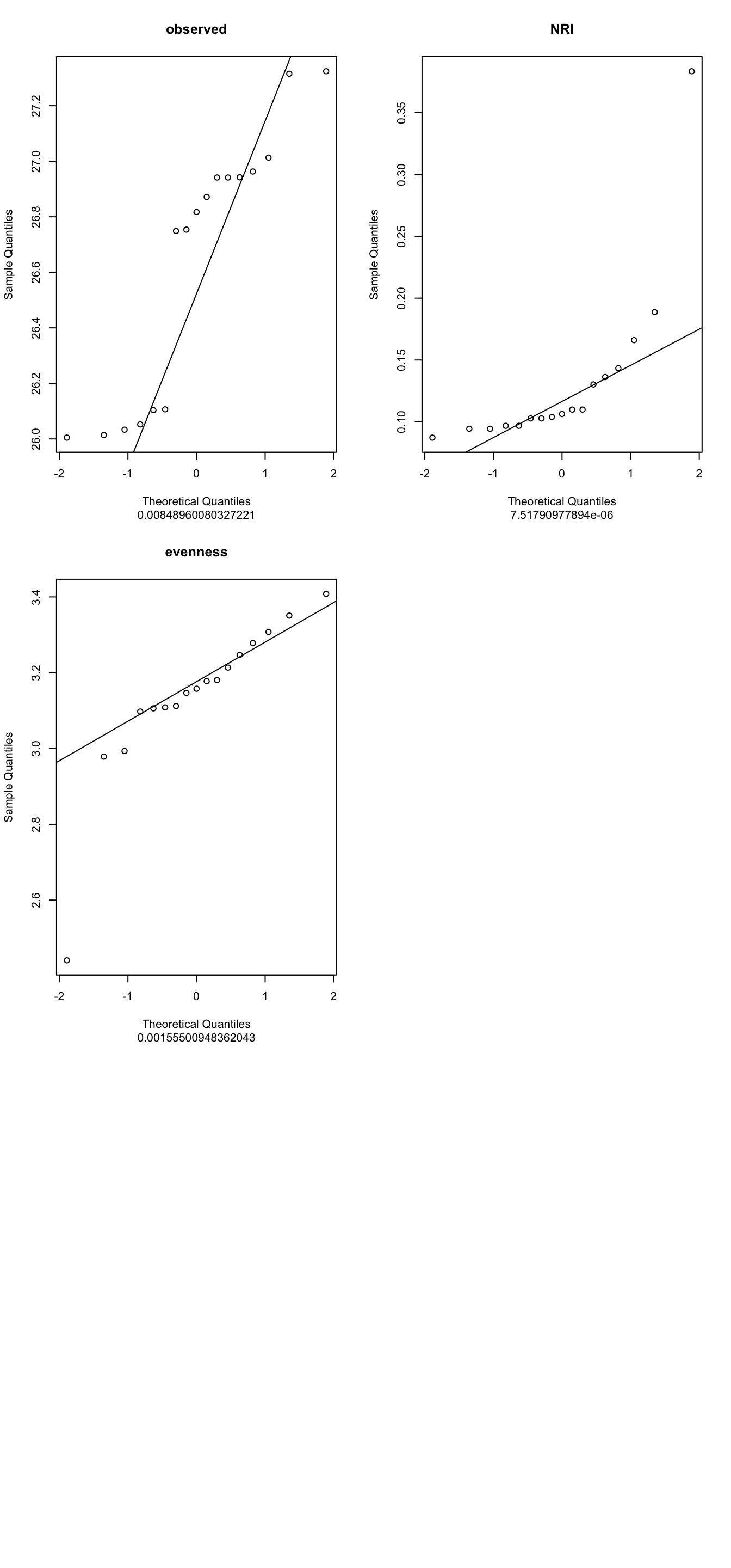

4- What are your conclusions?

5- PLease can you run a new normality test Using the parameters NO2,NO3,NH4,PO4 from the alldata object

c/ The ANOVA test

ANOVA is parametric (MUST follows normal distribution) AND run at least with 3 groups or more on ONE variable

_____________________________________
The procedure is :
Check Normality
Check homogeneity of variance
Apply ANOVA test (global test)
Apply Post-hoc Test (pairwise group test)
_____________________________________
Select number of groups

# How many groups used? See the column "groupe" of alldata (4 groups A,B,C,D):
factor(alldata$groupe)

 [1] C C C C D D D D D A A A A B B B B
Levels: A B C D

# Check homogeneity of variance between groups
# (this is to avoid bias in ANOVA result & keep the power of the test)
# H0= equality of variances in the different populations
bartlett.test(NH4 ~ groupe, alldata)


    Bartlett test of homogeneity of variances

data:  NH4 by groupe
Bartlett's K-squared = 6.8824, df = 3, p-value = 0.07574

6- Conclusion?
7- Why I can apply ANOVA on NH4 data?

NB: Alternative to Bartlett : Levene test (package car), less sensitive to normality deviation

Apply ANOVA global test
IMPORTANT: Global Test: Anova tell you if that some of the group means are different, but you don’t know which pairs of groups are different!

#Global test
aov_NH4 = aov(NH4 ~ groupe, alldata)
summary(aov_NH4)

            Df Sum Sq Mean Sq F value Pr(>F)  
groupe       3 0.3623 0.12076   3.482 0.0473 *
Residuals   13 0.4509 0.03469                 
---
Signif. codes:  0 '***' 0.001 '**' 0.01 '*' 0.05 '.' 0.1 ' ' 1

Apply Post-hoc test
IMPORTANT Anova told you that there is a significant difference between some groups… but Which pairs of groups are different? -> Post-hoc test answers this: Tukey multiple pairwise-comparisons

#Pairwise-comparisons
signif_pairgroups = TukeyHSD(aov_NH4, method = "bh")
signif_pairgroups

  Tukey multiple comparisons of means
    95% family-wise confidence level

Fit: aov(formula = NH4 ~ groupe, data = alldata)

$groupe
        diff        lwr         upr     p adj
B-A  0.13175 -0.2547839  0.51828386 0.7518486
C-A -0.15025 -0.5367839  0.23628386 0.6720556
D-A -0.24600 -0.6126982  0.12069822 0.2486076
C-B -0.28200 -0.6685339  0.10453386 0.1913308
D-B -0.37775 -0.7444482 -0.01105178 0.0426827
D-C -0.09575 -0.4624482  0.27094822 0.8680713

Representation of tukey results

plot(TukeyHSD(aov_NH4, conf.level=.95), las = 2)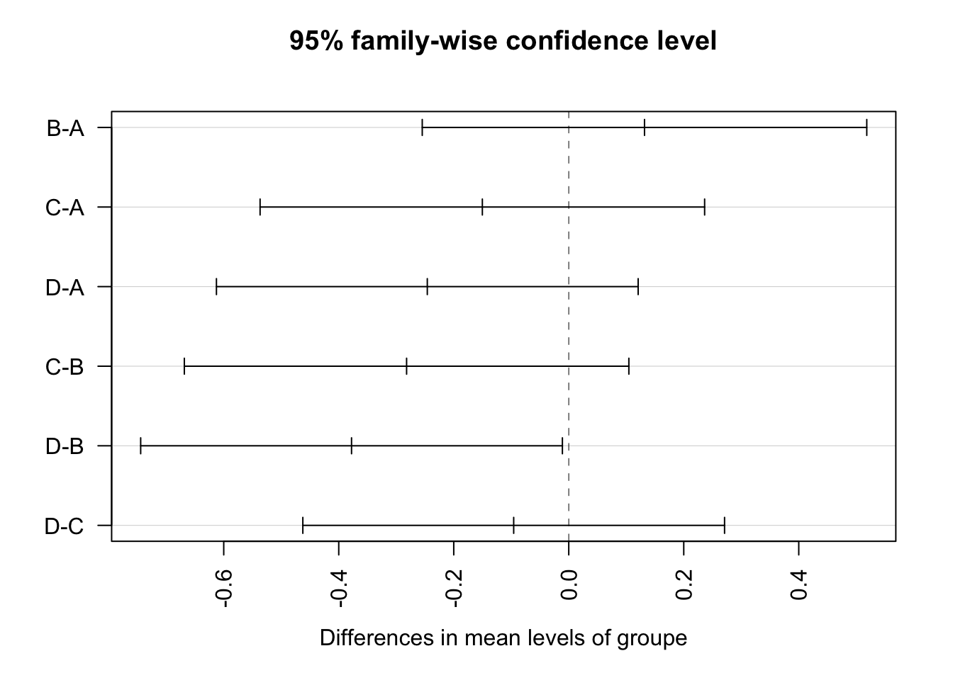

Tibble table: Reformate the output statistical test for use it with graphics

convert_format_Tukey = broom::tidy(signif_pairgroups)
convert_format_Tukey

# A tibble: 6 × 7
  term   contrast null.value estimate conf.low conf.high adj.p.value
  <chr>  <chr>         <dbl>    <dbl>    <dbl>     <dbl>       <dbl>
1 groupe B-A               0   0.132    -0.255    0.518       0.752 
2 groupe C-A               0  -0.150    -0.537    0.236       0.672 
3 groupe D-A               0  -0.246    -0.613    0.121       0.249 
4 groupe C-B               0  -0.282    -0.669    0.105       0.191 
5 groupe D-B               0  -0.378    -0.744   -0.0111      0.0427
6 groupe D-C               0  -0.0957   -0.462    0.271       0.868

split the column “contrast” into group1 et group2 (need for applying graph with p-values)

convert_format_Tukey = separate(convert_format_Tukey,contrast, c('group1', 'group2'),sep = "-")
convert_format_Tukey

# A tibble: 6 × 8
  term   group1 group2 null.value estimate conf.low conf.high adj.p.value
  <chr>  <chr>  <chr>       <dbl>    <dbl>    <dbl>     <dbl>       <dbl>
1 groupe B      A               0   0.132    -0.255    0.518       0.752 
2 groupe C      A               0  -0.150    -0.537    0.236       0.672 
3 groupe D      A               0  -0.246    -0.613    0.121       0.249 
4 groupe C      B               0  -0.282    -0.669    0.105       0.191 
5 groupe D      B               0  -0.378    -0.744   -0.0111      0.0427
6 groupe D      C               0  -0.0957   -0.462    0.271       0.868

Add a useful column

convert_format_Tukey$p.adj.signif = c("ns","ns","ns","ns","*","ns")
convert_format_Tukey

# A tibble: 6 × 9
  term   group1 group2 null.value estimate conf.low conf.high adj.p.value
  <chr>  <chr>  <chr>       <dbl>    <dbl>    <dbl>     <dbl>       <dbl>
1 groupe B      A               0   0.132    -0.255    0.518       0.752 
2 groupe C      A               0  -0.150    -0.537    0.236       0.672 
3 groupe D      A               0  -0.246    -0.613    0.121       0.249 
4 groupe C      B               0  -0.282    -0.669    0.105       0.191 
5 groupe D      B               0  -0.378    -0.744   -0.0111      0.0427
6 groupe D      C               0  -0.0957   -0.462    0.271       0.868 
# ℹ 1 more variable: p.adj.signif <chr>

Add another useful column

#Build column "custom.label" with condition
convert_format_Tukey$custom.label = ifelse(convert_format_Tukey$adj.p.value <= 0.05, convert_format_Tukey$adj.p.value,"ns")# replace convert_format_Tukey1 par convert_format_Tukey
convert_format_Tukey

# A tibble: 6 × 10
  term   group1 group2 null.value estimate conf.low conf.high adj.p.value
  <chr>  <chr>  <chr>       <dbl>    <dbl>    <dbl>     <dbl>       <dbl>
1 groupe B      A               0   0.132    -0.255    0.518       0.752 
2 groupe C      A               0  -0.150    -0.537    0.236       0.672 
3 groupe D      A               0  -0.246    -0.613    0.121       0.249 
4 groupe C      B               0  -0.282    -0.669    0.105       0.191 
5 groupe D      B               0  -0.378    -0.744   -0.0111      0.0427
6 groupe D      C               0  -0.0957   -0.462    0.271       0.868 
# ℹ 2 more variables: p.adj.signif <chr>, custom.label <chr>

build Boxplot with p-value

#boxplot
mygraph=ggplot(alldata, aes(x = groupe, y = NH4)) +
geom_boxplot(aes(color = groupe, fill = groupe))
mygraph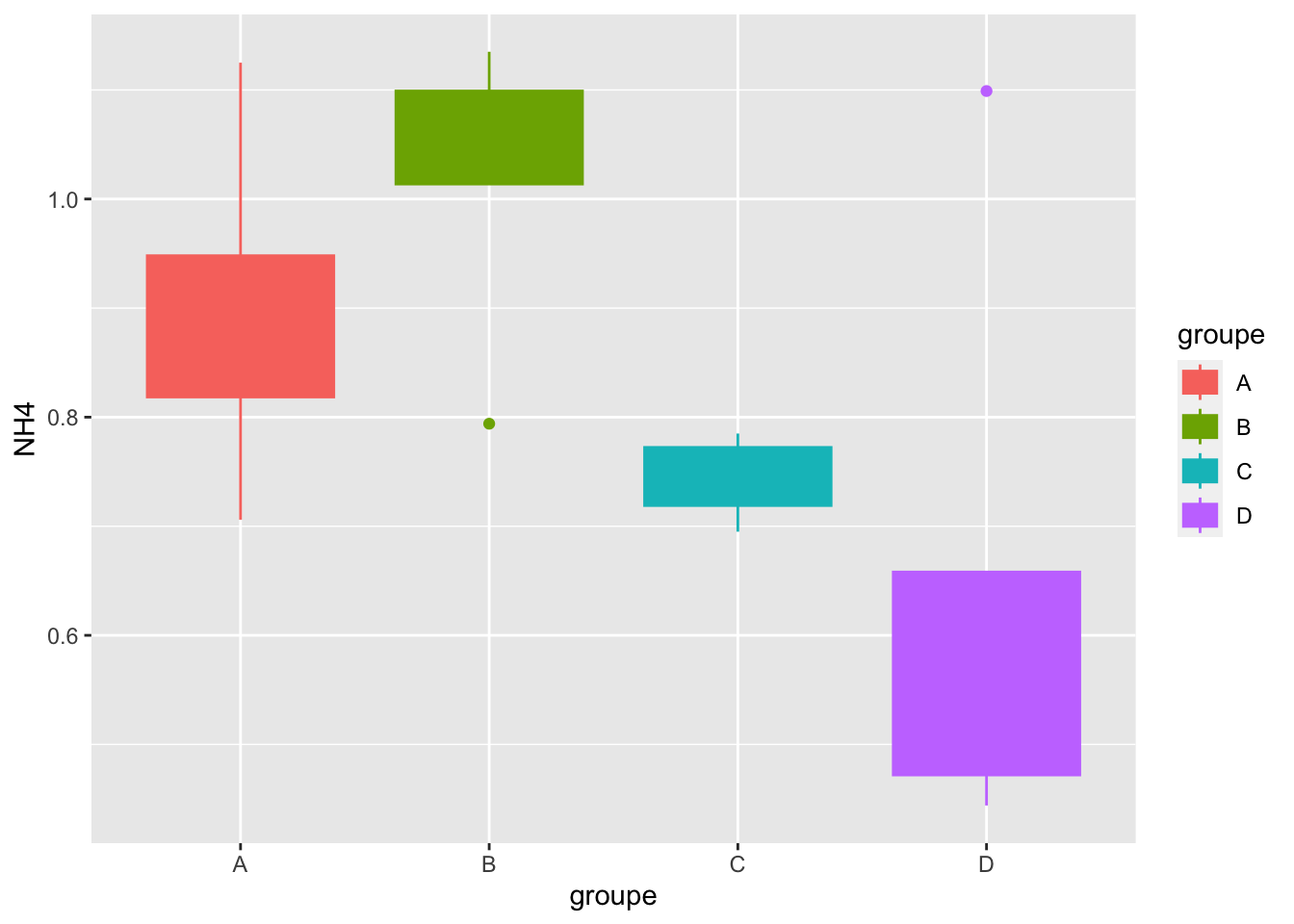

Geom_bracket() : Add p-values on graph

mygraph + 
geom_bracket(
aes(xmin = group1, xmax = group2, label = round(adj.p.value,2)),
data=convert_format_Tukey, y.position = 1.25,step.increase = 0.1,
tip.length = 0.01, color="blue")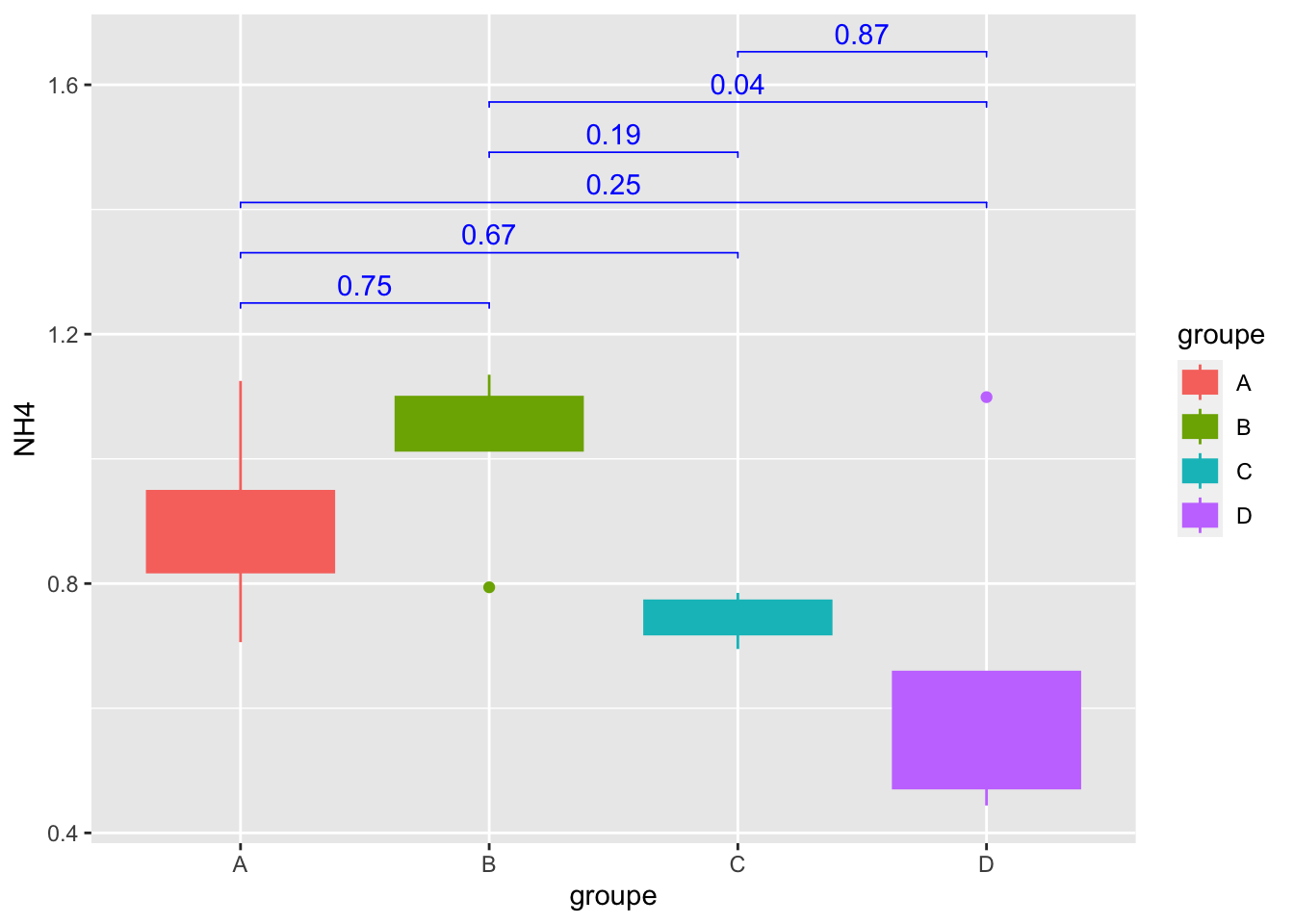

Geom_bracket() : Add significance on graph

mygraph + 
geom_bracket(
aes(xmin = group1, xmax = group2, label = p.adj.signif),
data=convert_format_Tukey, y.position = 1.25,step.increase = 0.1,
tip.length = 0.01, color="blue")

Geom_bracket() :Specify One or multiple brackets manually

mygraph + 
geom_bracket(
xmin = c("B","A"), xmax = c("D","C"), label = c("*","ns"),
y.position = 1.5,step.increase = 0.1,
tip.length = 0.01, color="blue")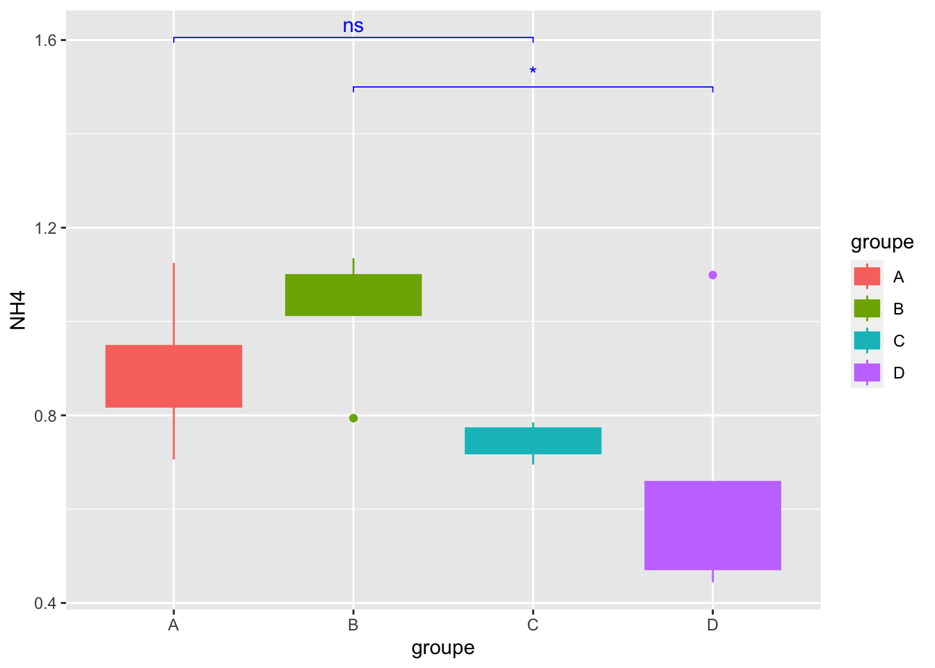

8- Conclusion about the statistical tests for NH4??
9- Now, do it for another Chemical parameter that follows normality…(Remember that you have check normality for other parameters see question -5)

d/ Kruskal-Wallis

Warning

IMPORTANT: IS non-parametric (for data not following normal distribution) & run at least on THREE or more groups for ONE variable

________________________________________________________
Procedure is :
- Apply Kruskal GLobal test
- Apply Post-hoc Test (pairwise group test, here Dunn)
________________________________________________________

Apply Kruskal-Wallis global test

kruskal.test(NO3 ~ groupe, data = alldata)


    Kruskal-Wallis rank sum test

data:  NO3 by groupe
Kruskal-Wallis chi-squared = 7.4994, df = 3, p-value = 0.05757

10- Why I’m using NO3?

Apply Post hoc test: Dunn test (pairwise group test)

signifgroup = dunnTest(NO3 ~ groupe,
                           data = alldata,
                           method = "bh")

Warning: groupe was coerced to a factor.

#See
signifgroup

Dunn (1964) Kruskal-Wallis multiple comparison

  p-values adjusted with the Benjamini-Hochberg method.

  Comparison         Z    P.unadj      P.adj
1      A - B  1.401139 0.16117254 0.32234509
2      A - C -1.120911 0.26232570 0.39348855
3      B - C -2.522050 0.01166731 0.07000387
4      A - D -0.738465 0.46023191 0.55227829
5      B - D -2.215395 0.02673296 0.08019887
6      C - D  0.443079 0.65770858 0.65770858

11- Conclusion??
12- Do you think that it was necessary to make the Post-hoc test? why?
13- Add a new categorical variable (=not numerical, exple the groupe column) in the table that allows forming 3 groups
14- Use NRI numerical variable and run Kruskal test with your new categorical variable, post-hoc test & boxblot representation

e/ T-test

Warning

IMPORTANT: Test is parametric= follow normal distribution,homogeneity of variance & run on 2 groups (ONE variable)

Select the groups

#Geo column
factor(alldata$Geo)

 [1] EU  EU  EU  EU  EU  EU  EU  EU  EU  USA USA USA USA USA USA USA USA
Levels: EU USA

Check homogeneity of variance

bartlett.test(PO4 ~ Geo, alldata)


    Bartlett test of homogeneity of variances

data:  PO4 by Geo
Bartlett's K-squared = 1.8936, df = 1, p-value = 0.1688

15- Can I run t-test according to homogeneity of variance result?Why?

#run t-test
observed_ttest = t.test(PO4 ~ Geo, data = alldata)
#see result
observed_ttest


    Welch Two Sample t-test

data:  PO4 by Geo
t = 2.8078, df = 13.108, p-value = 0.01471
alternative hypothesis: true difference in means between group EU and group USA is not equal to 0
95 percent confidence interval:
 0.03408592 0.26074742
sample estimates:
 mean in group EU mean in group USA 
        0.5036667         0.3562500

16- Conclusion?

f/ Wilcoxon rank-sum test

Warning

IMPORTANT: Is non-parametric (not follow normal distrib) & runs on 2 Groups and ONE variable

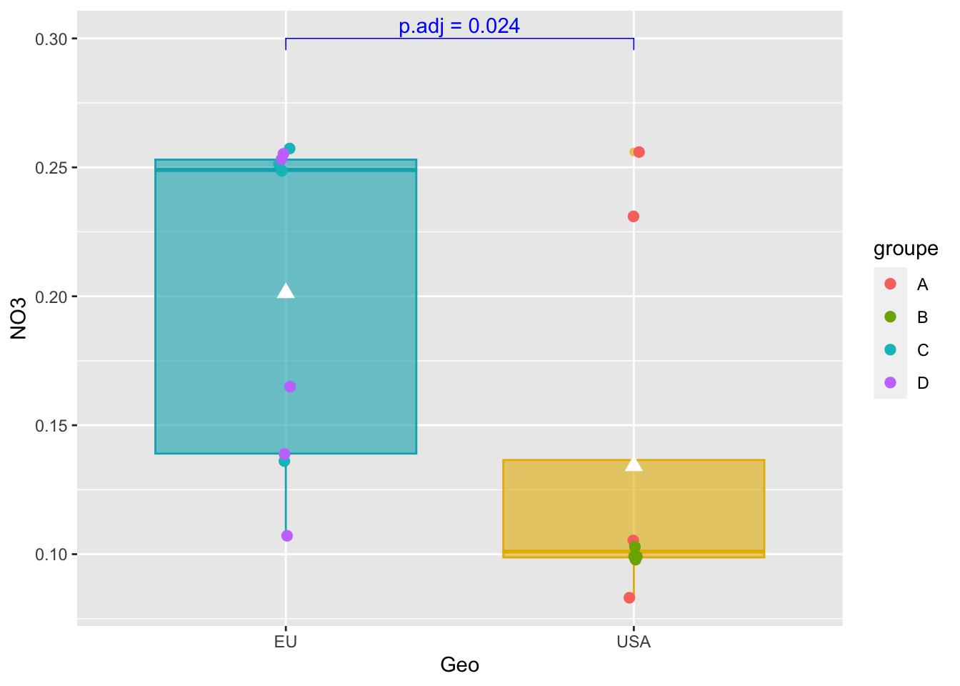
pairwise_test = compare_means(NO3 ~ Geo,
                                       alldata,
                                       method = "wilcox.test")
#See
pairwise_test

# A tibble: 1 × 8
  .y.   group1 group2      p p.adj p.format p.signif method  
  <chr> <chr>  <chr>   <dbl> <dbl> <chr>    <chr>    <chr>   
1 NO3   EU     USA    0.0237 0.024 0.024    *        Wilcoxon

17- Why the choice of NO3? Conclusion?

Boxplot representation with p-value using stat_pvalue_manual

#Boxplot as previously seen
graph_shan = ggplot(alldata, aes(x = Geo, y = NO3)) + 
  geom_boxplot(alpha=0.6,
               fill = c("#00AFBB", "#E7B800"),
               color = c("#00AFBB", "#E7B800")) +
  geom_jitter(aes(colour = groupe),
              position = position_jitter(0.02) ,
              cex=2.2) +
  stat_summary(fun = mean, geom = "point",
               shape = 17, size = 3,
               color = "white")
#see
graph_shan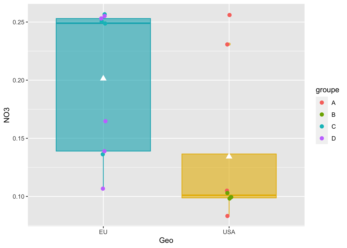

Add p-value on graph

graph_shan + stat_pvalue_manual(
  pairwise_test,
  y.position = 0.3,
  label = "p.adj = {p.adj}",
  color = "blue",
  linetype = 1,
  tip.length = 0.02
)

IV- Bivariate Analysis

________________________________________________________________
Study the relationship between two variables (quantitatives or qualitatives)
________________________________________________________________

A- Correlation analysis

Important : Correlation coefficient r is independent of change of origin and scale (So no data transformation!!)
Correlation analysis describes the nature (strength (0 to 1) and direction Positive/Negative) of the relationship between two quantitative variables (r),whatever the range and the measurement units of them.
___________________________
Methods & conditions :
- Pearson : Parametric
- Spearman: Non-Parametric
- Kendall : Non-parametric
___________________________
The procedure is :
- Select your variables of interest
- Test the Normality of data
- Choose the right method according Normality result
- Apply Correlation method
- Apply statistical test
- Build the final plot
___________________________

a1/ Select variables that you want

#Select variables for bivariate correlation
myvariables = select(alldata, SiOH4:PO4, observed,PD)
#see
myvariables

   SiOH4   NO2   NO3   NH4   PO4 observed          PD
1    945 2.669 0.136 0.785 0.267  26.1065  1.95798975
2   1295 2.206 0.249 0.768 0.629  27.3241  1.11902329
3   1300 3.004 0.251 0.727 0.653  27.3151 -0.01038346
4   1600 3.016 0.257 0.695 0.491  26.7536 -0.64181960
5   1355 1.198 0.165 1.099 0.432  26.7488  0.79285403
6   1590 3.868 0.253 0.567 0.533  26.9423  0.81104335
7   2265 3.639 0.255 0.658 0.665  26.8713  0.51096388
8   1180 3.910 0.107 0.472 0.490  27.0131  0.26352612
9   1545 3.607 0.139 0.444 0.373  26.8172  2.43432750
10  1690 2.324 0.083 0.856 0.467  26.9631 -1.62669669
11   115 1.813 0.256 0.889 0.324  26.0046 -0.75543498
12   395 2.592 0.105 1.125 0.328  26.0521 -0.69141166
13   395 2.381 0.231 0.706 0.450  26.0137 -0.64705490
14   200 1.656 0.098 0.794 0.367  26.0332 -0.67857965
15   235 2.457 0.099 1.087 0.349  26.9415  0.05055793
16   235 2.457 0.099 1.087 0.349  26.9415 -0.84513858
17  1355 2.028 0.103 1.135 0.216  26.1037  0.12211753

a2/ Normality

indices_normality(myvariables, nrow =3, ncol = 3)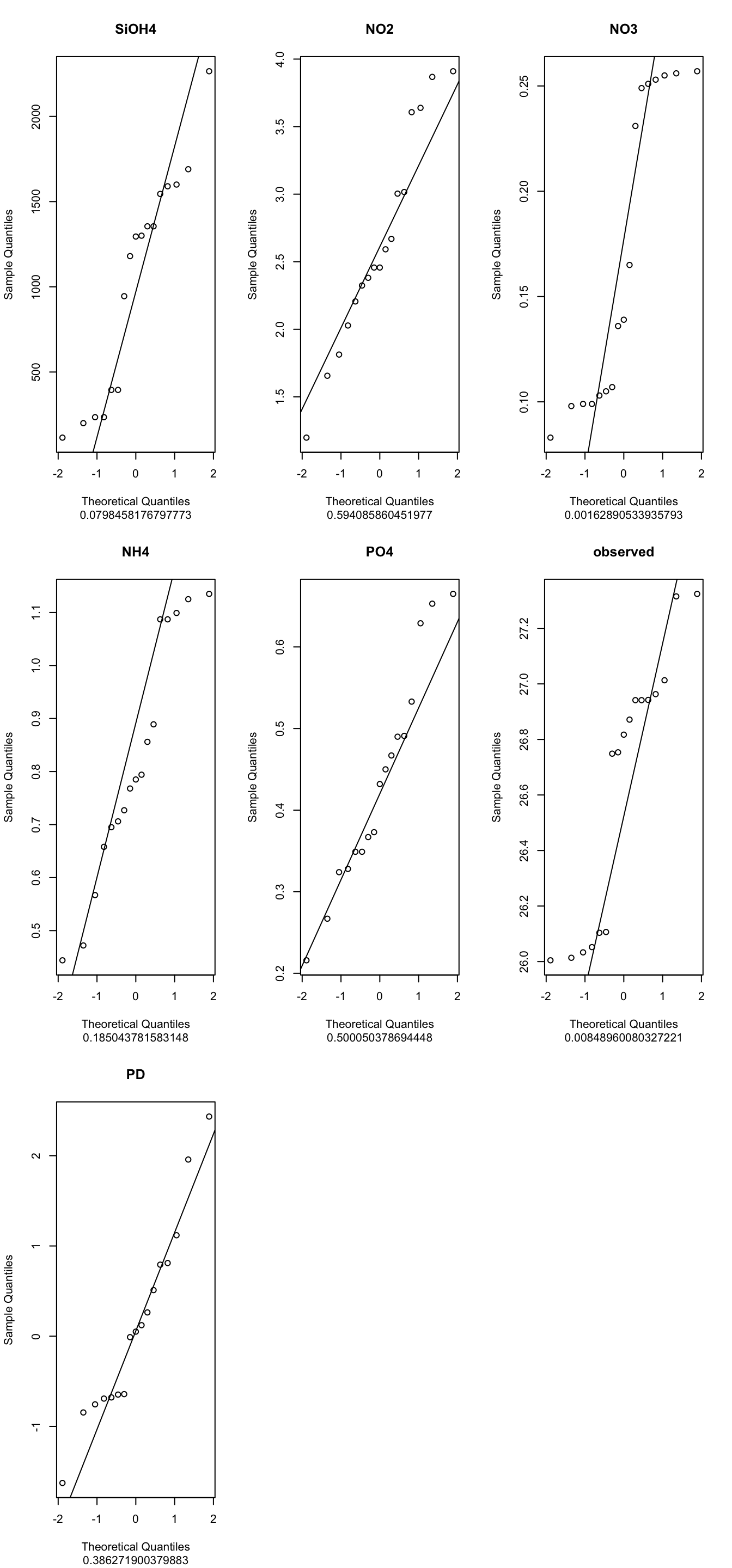

18- <span style=“color: red;”Conclusions, which method to apply?

a3/ Apply the Pearson method

#Apply method pearson
matrixCor = cor(myvariables, method = "pearson")
#see
matrixCor

              SiOH4        NO2        NO3        NH4         PO4   observed
SiOH4     1.0000000  0.4856257  0.3140398 -0.4513788  0.56085793  0.5066938
NO2       0.4856257  1.0000000  0.2124683 -0.7269246  0.41715983  0.4170527
NO3       0.3140398  0.2124683  1.0000000 -0.4036942  0.63751606  0.1928259
NH4      -0.4513788 -0.7269246 -0.4036942  1.0000000 -0.51338488 -0.2944559
PO4       0.5608579  0.4171598  0.6375161 -0.5133849  1.00000000  0.7054092
observed  0.5066938  0.4170527  0.1928259 -0.2944559  0.70540919  1.0000000
PD        0.3665477  0.3343467  0.1300303 -0.3958036  0.04168105  0.1832832
                  PD
SiOH4     0.36654770
NO2       0.33434675
NO3       0.13003033
NH4      -0.39580362
PO4       0.04168105
observed  0.18328322
PD        1.00000000

Save the table with correlation values

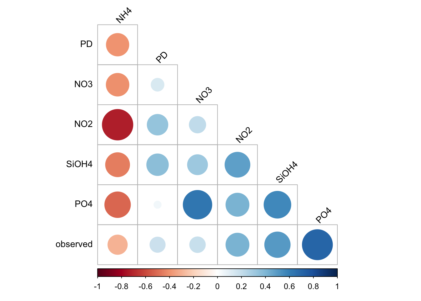
write.table(matrixCor,file="./correlation_matrix.txt",sep = "\t")

a4/ Plot results: corrplot function

corrplot(
  matrixCor,
  method="circle",
  type="lower",
  order='hclust',
  tl.col = "black",
  tl.srt = 45,
  tl.cex=0.9,
  diag = FALSE
)

a5/ Is the correlation is due to chance? Significance test!
______________________________________________________
The idea:
Test the correlation at the population scale (= increase data , it’s call Rho) and compare to r (your samples)
H0 is : There is no significant linear correlation between X and Y variables in the population
For instance a t-test allows to use sample data to generalize an assumption to an entire population
______________________________________________________

#Test stats
ptest =cor.mtest(matrixCor, conf.level = .95)

#ptest is a list... see 
class(ptest)

[1] "list"

#See the list
ptest

$p
              SiOH4        NO2        NO3        NH4        PO4   observed
SiOH4    0.00000000 0.03104693 0.23694105 0.01713865 0.04594221 0.06146485
NO2      0.03104693 0.00000000 0.30094151 0.00110837 0.09506126 0.10206651
NO3      0.23694105 0.30094151 0.00000000 0.09663095 0.03311411 0.39456306
NH4      0.01713865 0.00110837 0.09663095 0.00000000 0.03715039 0.10437538
PO4      0.04594221 0.09506126 0.03311411 0.03715039 0.00000000 0.01782655
observed 0.06146485 0.10206651 0.39456306 0.10437538 0.01782655 0.00000000
PD       0.23167149 0.18000316 0.73582000 0.12998482 0.77570253 0.65179758
                PD
SiOH4    0.2316715
NO2      0.1800032
NO3      0.7358200
NH4      0.1299848
PO4      0.7757025
observed 0.6517976
PD       0.0000000

$lowCI
               SiOH4        NO2        NO3        NH4         PO4    observed
SiOH4     1.00000000  0.1158642 -0.3889387 -0.9763259  0.02371354 -0.04704726
NO2       0.11586418  1.0000000 -0.4500231 -0.9926251 -0.15583006 -0.17380558
NO3      -0.38893869 -0.4500231  1.0000000 -0.9466621  0.10098312 -0.51886347
NH4      -0.97632595 -0.9926251 -0.9466621  1.0000000 -0.96636922 -0.94453657
PO4       0.02371354 -0.1558301  0.1009831 -0.9663692  1.00000000  0.23878062
observed -0.04704726 -0.1738056 -0.5188635 -0.9445366  0.23878062  1.00000000
PD       -0.38318235 -0.3185439 -0.6756654 -0.9378870 -0.68891124 -0.64526193
                 PD
SiOH4    -0.3831823
NO2      -0.3185439
NO3      -0.6756654
NH4      -0.9378870
PO4      -0.6889112
observed -0.6452619
PD        1.0000000

$uppCI
              SiOH4        NO2       NO3         NH4         PO4  observed
SiOH4     1.0000000  0.9690429 0.9136889 -0.24712040  0.96285638 0.9573268
NO2       0.9690429  1.0000000 0.9005713 -0.68559598  0.94710076 0.9451638
NO3       0.9136889  0.9005713 1.0000000  0.15996568  0.96811152 0.8821061
NH4      -0.2471204 -0.6855960 0.1599657  1.00000000 -0.07415082 0.1794714
PO4       0.9628564  0.9471008 0.9681115 -0.07415082  1.00000000 0.9759077
observed  0.9573268  0.9451638 0.8821061  0.17947138  0.97590766 1.0000000
PD        0.9147994  0.9260528 0.8140329  0.23527330  0.80550109 0.8314534
                PD
SiOH4    0.9147994
NO2      0.9260528
NO3      0.8140329
NH4      0.2352733
PO4      0.8055011
observed 0.8314534
PD       1.0000000

#to see only the p-values you must call ptest$p
ptest$p

              SiOH4        NO2        NO3        NH4        PO4   observed
SiOH4    0.00000000 0.03104693 0.23694105 0.01713865 0.04594221 0.06146485
NO2      0.03104693 0.00000000 0.30094151 0.00110837 0.09506126 0.10206651
NO3      0.23694105 0.30094151 0.00000000 0.09663095 0.03311411 0.39456306
NH4      0.01713865 0.00110837 0.09663095 0.00000000 0.03715039 0.10437538
PO4      0.04594221 0.09506126 0.03311411 0.03715039 0.00000000 0.01782655
observed 0.06146485 0.10206651 0.39456306 0.10437538 0.01782655 0.00000000
PD       0.23167149 0.18000316 0.73582000 0.12998482 0.77570253 0.65179758
                PD
SiOH4    0.2316715
NO2      0.1800032
NO3      0.7358200
NH4      0.1299848
PO4      0.7757025
observed 0.6517976
PD       0.0000000

19- Save the result in a file
20- Can you display only the value of PD column of ptest$p (help: first check the class of ptest$p)?

a6/ Plot only correlations with significant p-values

corrplot(
  matrixCor,
  p.mat = ptest$p,
  sig.level = .05,
  method = "circle",
  type = "lower",
  order = 'hclust',
  tl.col = "black",
  tl.srt = 45,
  tl.cex = 0.7,
  diag = FALSE
)

B- Linear regression

______________________________________________________________________
Determination of coefficient R² provides percentage variation in Y which is explained by all the X together.
Its value is (usually) between 0 and 1 and it indicates strength of Linear Regression model.
- High R² value, data points are less scattered so it is a good model
- Low R² value is more scattered the data points
______________________________________________________________________

b1/ Regression Shannon ~ Observed

ggplot(alldata, aes(x = observed, y = shannon)) +
  geom_point() +
  stat_smooth(method = "lm", col = "red") +
  stat_poly_eq(aes(label = paste(after_stat(rr.label),
                                          after_stat(p.value.label),
                                          sep = "*\", \"*")))

`geom_smooth()` using formula = 'y ~ x'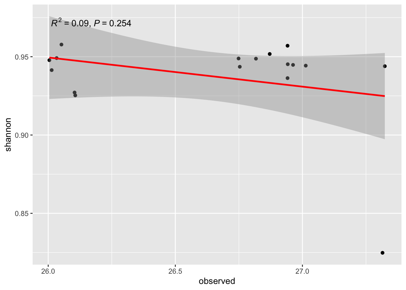

21- What is the question we try to answer?
22- Conclusion?

b2/ Linear Regression NH4 ~ NO2

ggplot(alldata, aes(x = NO2, y = NH4)) +
  geom_point() +
  stat_smooth(method = "lm", col = "red") +
  stat_poly_eq(aes(label = paste(after_stat(rr.label),
                                          after_stat(p.value.label),
                                          sep = "*\", \"*")))

`geom_smooth()` using formula = 'y ~ x'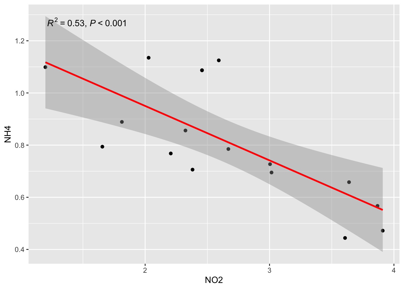

23- What are √R² of this exemple? See matrixCor… Do you see the relation beetween R² and r?

if you not see, try to run in the console: cor(alldata$NH4, alldata$NO2)

BUT

Remember that you have two population groups (EU vs USA) in the data

ggplot(alldata, aes(x = NO2, y = NH4, col=Geo)) +
  geom_point() +
  stat_smooth(method = "lm", col = "red") +
  stat_poly_eq(aes(label = paste(after_stat(rr.label),
                                          after_stat(p.value.label),
                                          sep = "*\", \"*")))

`geom_smooth()` using formula = 'y ~ x'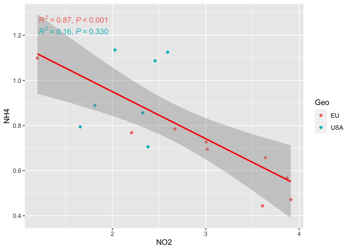

AND MORE…
facet_grid option to separate the two graph

ggplot(alldata, aes(x = NO2, y = NH4, col=Geo)) +
  geom_point() +
  stat_smooth(method = "lm", col = "red") +
  stat_poly_eq(aes(label = paste(after_stat(rr.label),
                                          after_stat(p.value.label),
                                          sep = "*\", \"*")))+
  facet_grid(rows=vars(Geo))

`geom_smooth()` using formula = 'y ~ x'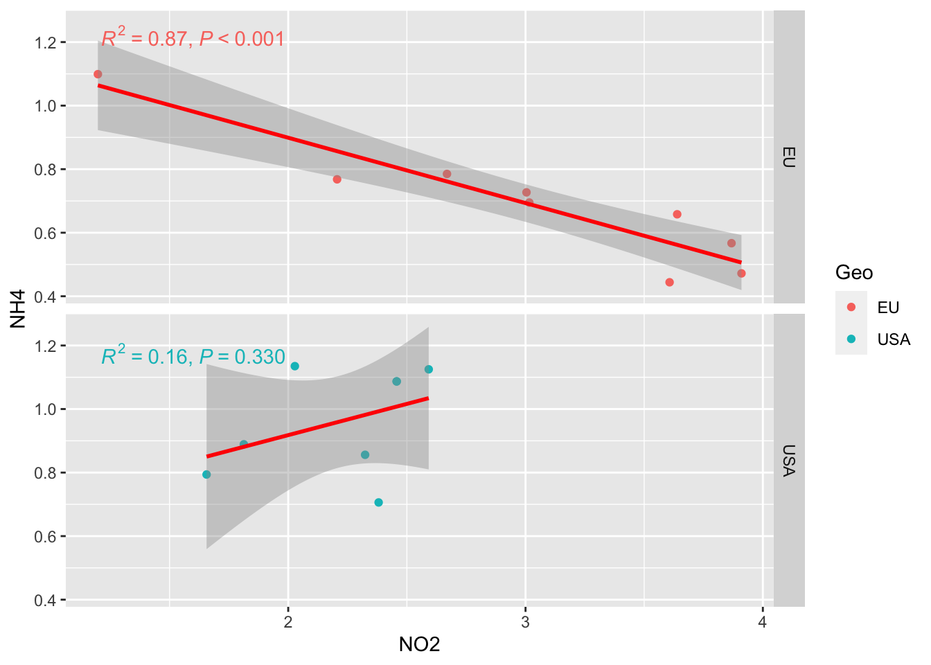

BONUS
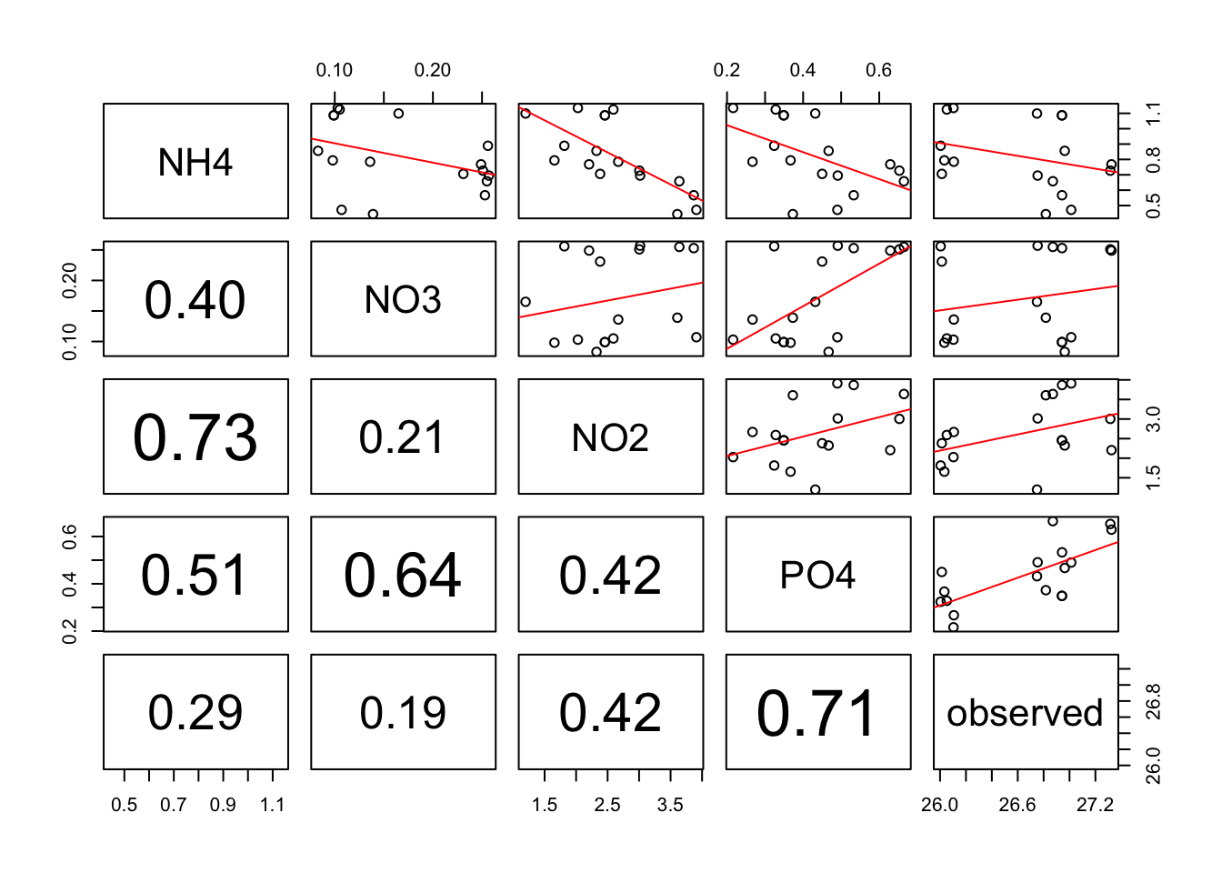
Make linear regression + add correlation r coeficent for numerous variable in ONE step!!
Allow you to rapidely see wich variables are correlated among a huge list.

pairs(alldata[, c("NH4","NO3", "NO2","PO4", "observed")],upper.panel = regression_line, lower.panel=panel.cor)

Warning in par(usr): argument 1 does not name a graphical parameter

Warning in par(usr): argument 1 does not name a graphical parameter

Warning in par(usr): argument 1 does not name a graphical parameter

Warning in par(usr): argument 1 does not name a graphical parameter

Warning in par(usr): argument 1 does not name a graphical parameter

Warning in par(usr): argument 1 does not name a graphical parameter

Warning in par(usr): argument 1 does not name a graphical parameter

Warning in par(usr): argument 1 does not name a graphical parameter

Warning in par(usr): argument 1 does not name a graphical parameter

Warning in par(usr): argument 1 does not name a graphical parameter

Load libraries & functions

I- Manipulate a data table

a/ Read a table containing data

b/ Select a subset from data table

c/ How to Add a new variable after loading table

Merge the two dataframes!

II- Descriptive statistics

a/ Get stats info for all variables

b/ Get stats info by groups

c/ Distribution plot

III- Inferential Statistics & Tests

a/ Select indices to test & run normality check : select function

b/ Run Normality test: QQ-plot +Shapiro

c/ The ANOVA test

ANOVA is parametric (MUST follows normal distribution) AND run at least with 3 groups or more on ONE variable

Select number of groups

Apply ANOVA global test

Apply Post-hoc test

Representation of tukey results

Tibble table: Reformate the output statistical test for use it with graphics

split the column “contrast” into group1 et group2 (need for applying graph with p-values)

Add a useful column

Add another useful column

build Boxplot with p-value

Geom_bracket() : Add p-values on graph

Geom_bracket() : Add significance on graph

Geom_bracket() :Specify One or multiple brackets manually

d/ Kruskal-Wallis

Apply Kruskal-Wallis global test

Apply Post hoc test: Dunn test (pairwise group test)

e/ T-test

Select the groups

Check homogeneity of variance

f/ Wilcoxon rank-sum test

Boxplot representation with p-value using stat_pvalue_manual

Add p-value on graph

IV- Bivariate Analysis

A- Correlation analysis

a1/ Select variables that you want

a2/ Normality

a3/ Apply the Pearson method

Save the table with correlation values

a4/ Plot results: corrplot function

a5/ Is the correlation is due to chance? Significance test!

a6/ Plot only correlations with significant p-values

B- Linear regression

b1/ Regression Shannon ~ Observed

b2/ Linear Regression NH4 ~ NO2

BUT

AND MORE…

BONUS